The Appraisal Process and Land Valuation
Land should be valued by incorporating the steps of the appraisal process. In this way, all sources of appraisal information will have been explored and the final estimate of value will reflect a justifiable and defensible conclusion based on this appraisal information.
The steps in the appraisal process are as follows:
- Definition of the problem
- Preliminary survey and planning
- Data collection and analysis
- Application of the approaches to value
- Reconciliation of value estimates
- Final estimate of value
Definition of the Problem
Beginning the land valuation process requires that the appraiser define the problem, the solution to which is the objective of the appraisal. In defining the problem, the appraiser needs to determine the following, prior to beginning the appraisal:
- Identification of the subject property or properties
- Property rights involved
- Date of appraisal and assessment date and level of value
- Purpose and function of the appraisal
- Definition of value
Identification of the Subject Property
Identification of the property can be provided by a street address, legal description or parcel identification number. Additional information about property identification may be found in ARL Volume 2, Administrative and Assessment Procedures, Chapter 13, Land Identification and Real Property Descriptions, and Chapter 14, Assessment Mapping and Parcel Identification.
Property Rights Involved
Colorado statute § 39-1-103(5)(a), C.R.S., requires that the fee simple estate be valued for property tax purposes. This requirement is confirmed by § 39-1-106, C.R.S., - the Unit Assessment Rule. Market value of the fee simple estate should reflect market assumptions, including market rent, market expenses, and market occupancy. For most real property interests, Colorado assessors are required by §§ 39-1-106 and 39-5-102(1), C.R.S., to assess land to the owner of record. The appraiser should be aware that fractional ownership interests in land may exist and those interests should be identified during the definition of the problem step in the appraisal process.
Possessory interests in exempt land may exist. Refer to Chapter 7, Special Issues in Valuation, under Assessment of Possessory Interest, for classification and valuation procedures for possessory interests.
Date of Appraisal and Assessment Date
The date of appraisal is June 30 of the year preceding the year of general reappraisal. All applicable approaches to appraisal must be trended or adjusted to this date.
Colorado statute § 39-1-105, C.R.S., provides that the date of assessment is to be January 1 each year and that all property is to be listed as it exists in the county where it is located on the assessment date.
To distinguish between the two dates, the assessment date refers to the date upon which property situs (location), taxable status, and the property's physical characteristics are established for that assessment year, while the appraisal date refers to the date upon which the valuation of the property is based or otherwise adjusted or trended.
For additional information on the appraisal date and the data collection period, please refer to Chapter 3, Sales Confirmation and Stratification.
Purpose and Function of the Appraisal
The purpose of the land appraisal is to estimate value. The function of the land appraisal refers to the reason that the appraisal was created, i.e., as a basis for property taxation.
Definition of Value
Other than very generally in §§ 39-1-103(5)(a) and 104(10.2)(d), C.R.S., Colorado statutes do not provide a specific definition of actual value. However, there are a number of Colorado court cases that mention actual value and market value. In Fellows v. Grand Junction Sugar Co., 78 Colo. 393, 242 P. 635 (1925), the court concluded that "In determining ‘fair value’ or ‘actual value’, market value is usually taken as the measure, because it is most likely to be just and least difficult of ascertainment." Other Colorado cases such as Colorado & Utah Coal Co. v. Rorex, 149 Colo. 502, 369 P.2d 796 (1962) and May Stores Shopping Centers, Inc. v. Shoemaker, 151 Colo. 100, 376 P.2d 679 (1962) mention market value and attempt to define it.
The definition of market value developed by the Appraisal Institute is based on California case law: Sacramento Southern R.R. Co. v. Heilbron, 156 Cal. 408, 104 P. 979 (1909).
The Appraisal Institute market value definition derived from the above case is as follows:
"The most probable price, as of a specified date, in cash, or in terms equivalent to cash, or in other precisely revealed terms, for which the specified property rights should sell after reasonable exposure in a competitive market under all conditions requisite to a fair sale, with the buyer and seller each acting prudently, knowledgeably, and for self-interest, and assuming that neither is under undue duress."
Preliminary Survey and Planning
After definition of the appraisal problem, the appraiser must begin development of a plan for the appraisal. In developing the plan, an analysis of property uses must be completed.
There are basically two steps in preliminary survey and planning:
- Determination of the use of the property and an analysis of how actual use of the property relates to its highest and best use
- Development of the plan for the appraisal
Use Determination and Highest and Best Use
In developing a good land valuation program, the assessor must correctly classify land. The primary criterion for classification is the actual use of the land on the assessment date. When actual use cannot be determined through physical inspection, the property owner should be contacted. The assessor may also consider such things as zoning or use restrictions, historical use, or consistent use, in determining land use. When unable to determine actual use, the assessor may consider the land’s most probable use, as of the assessment date, based on the best information available.
Proper classification is also very important for abstract purposes. To ensure that each parcel has the proper coding, and for classification descriptions, refer to ARL Volume 2, Administrative and Assessment Procedures, Chapter 6, Property Classification Guidelines and Assessment Percentages. After reviewing the instructions and codes, land appraisers should enter the county's appropriate classification and subclassification code on each parcel's property record.
Proper land classification is essential in order to establish how the property is to be valued. Classification, based on actual use, should not be confused with determining value. Colorado statutes require that certain types of land be valued using variations on, or elimination of, one or more of the three approaches, i.e., the cost, market, or income approach, to value. Examples of this requirement would be in the valuation of residential improved land, agricultural land, oil and gas leaseholds and lands, and producing mines. Unless otherwise directed by law, the three approaches to value should be considered.
Valuation for ad valorem property taxation should be based on a property’s highest and best use. The requirement of valuing property at its highest and best use was affirmed by the Colorado Supreme Court in Board of Assessment Appeals, et al, v. Colorado Arlberg Club, 762 P.2d 146 (Colo. 1988). In that case the court concluded that “reasonable future use is relevant to a property’s current market value for tax assessment purposes.” The court further noted “our statute does not preclude consideration of future uses” and it quoted the American Institute of Real Estate Appraisers, referencing The Appraisal of Real Estate 33, 1983, 8th Edition, “In the market, the current value of a property is…based on what market participants perceive to be the future benefits of acquisition.” Reasonable future use is based on the actions and expectations of the market, and is consistent with the highest and best use concept that requires use to be physically possible, legally permissible, financially feasible, and maximally productive.
Economic Unit Analysis (AKA, Tie-Back Parcels)
Colorado Statute 39-5-104, titled Valuation of Property, states that “When a single structure, used for a single purpose, is located on more than one town or city lot, the entire land area shall be appraised and valued as a single property.” Also, the statute requires that these parcels are under the same ownership and are adjoining. This statute applies the economic unit concept as explained in the Dictionary of Real Estate Appraisal, 7th ed.: “A combination of parcels in which land and improvements are used for mutual economic benefit.” The Dictionary also notes that “identification of economic units is essential in highest and best use analysis.” A highest and best use analysis is the foundation of all appraisal and is the first step in identifying an economic unit. The Highest and Best Use analysis will answer the question whether an out parcel is part of the economic unit or instead is excess or surplus land. If it is determined that an out parcel is excess or surplus land, then it should be valued separate from the economic unit. On the other hand, if the out parcel is determined to be part of the economic unit, then its value is included as part of that unit. The overarching concept here is that these properties are valued as a unit rather than as the sum of the individual parcels that make up the economic unit. However for ad valorem appraisal a separate value must be assigned to each parcel that makes up the economic unit. Guidance from the Dictionary is only that each parcel must make a positive economic contribution to the unit. For fee appraisal this distinction is typically not an issue as the appraiser’s assignment is to value the economic unit. A common example of this situation is shopping centers that include out parcels that provide access or the required parking to meet market standards. (These out parcels are often referred to as tie-back parcels.) In this situation the market value of the shopping center, the economic unit, is established by consideration of the three approaches to value. Although most of this value is with the parent parcel, value must be assigned to each out parcel. A corresponding reduction must be made to the total market value of the center as reflected in the parent parcel, so that the economic unit is not overvalued.
Development of an Appraisal Plan
Development of a plan, especially when undertaking a mass appraisal of land, is essential in order to use available resources at maximum efficiency. Planning for an appraisal involves the following:
- Consider, determine, and document which approaches to value will be most appropriate.
In considering, determining, and documenting which valuation approach or approaches should be used, Colorado case law should be referenced.
Montrose Properties, LTD., et al., v. Colorado Board of Assessment Appeals, et al., 738 P.2d 396 (Colo. App. 1987) affirms § 39-1-103(5)(a), C.R.S., and defines the assessor's "appropriate consideration" of all required approaches to value. The court concluded that "appropriate consideration" was used by an assessor when the assessor decided that insufficient information precluded the use and calculation of one or more of the required approaches. The court reasoned appropriate consideration was used in determining the approach(es) that were not applicable. The need for appropriate consideration of the three approaches was affirmed by the Colorado Supreme Court in Board of Assessment Appeals, et al., v. Sonnenberg, 797 P.2d 27 (Colo. 1990).
Transamerica Realty Corporation v. Clifton, et al., 817 P.2d 1049 (Colo. App. 1991) requires the assessor to provide evidence to support adequate documentation of the values established for all applicable approaches to appraisal. Insufficient time is not a reasonable excuse for failure to consider the applicable approaches to appraisal.
These requirements have considerable current impact due to § 20 of article X of the Colorado Constitution removing the presumption of correctness from the assessor's values. Beginning January 1, 1993, valuation issues shall be decided based on the preponderance of the evidence.
- Determine what type of appraisal data must be gathered and what data sources are available.
- Determine resource requirements and allocate existing resources in a manner to complete a quality appraisal.
- Estimate the budget cost for the appraisal. If budgets have been previously set and additional funds are not available, the appraisal plan must be redrawn to fit into existing budget constraints.
Specific information on development of an appraisal plan may be found in ARL Volume 2, Administrative and Assessment Procedures, Chapter 2, Assessment Operations.
Data Collection and Analysis
Appraisal data that will be collected and analyzed will fall into one of three categories:
- General
- Specific
- Comparative
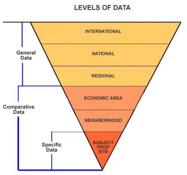
General data is an overall category that pertains to information about the four forces (physical, economic, governmental and social) originating outside a subject property and those forces' influence on that property's value. General data provides a background basis for analysis of international, national, and regional trends that affect value.
Examples of general data would be U.S. Census publications, U.S. Labor Department employment statistics, and Colorado Division of Housing information on construction costs and housing starts.
Specific data pertains primarily to information about the site. Examples of specific data would be title and recorded information such as legal description, special assessments, zoning, easements, other public restrictions, and physical information about the site.
Comparative data consists of cost, sales, and income information on individual properties. When properly screened and confirmed, comparative data is used directly in the cost, market, and income approaches to valuing the subject property.
Examples of comparative data are vacant land sales collected within the statutory data collection period as stated in § 39-1-104(10.2), C.R.S., development costs for comparable subdivisions, and economic rental rates.
Refer to the following diagram for a graphic representation of how general, specific, and comparative data are collected for various geographic areas.
Survey of Appraisal Information Sources
Data sources of appraisal information may be divided into two categories.
- Public records
- Private sources
The major sources of public records are found in the county courthouse.
The local county clerk is a source of information on the following:
- Documentary fee information for land sales
- "Real Property Transfer Declarations" (Form TD-1000) for deeds requiring documentary fees and recorded after July 1, 1989. “Manufactured Home Transfer Declarations" for titled manufactured homes that are conveyed after July 1, 2009. These are confidential
- Copies of recorded leases
- Land descriptions from recorded plats
- Other general data about the county and cities within the county
The local planning office is a good source of information on the following:
- Zoning
- Building codes
- Traffic patterns
- Water and sewer availability
- Other important data about the property
Private sources include the following:
- A subscription to the Multiple Listing Service sold book*
- Real estate agents' records
- Publications of all types
- Media advertising
- The local Chamber of Commerce office
- Other appraisers
- Title companies
- Mortgage banks
- Property managers
- University or college studies
- Other similar sources
*Provided by the local Realtor's Association.
Neighborhoods and Economic Areas
The following subsections refer to the development of neighborhoods and economic areas.
Economic Base Analysis
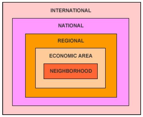
Economic base analysis is the evaluation of the supply of products produced and services delivered in a given area and the demand for these products in the local, regional, national, and international markets.
In the context of the appraisal process, the supply of and demand for various goods and services affect the value of real estate in the smallest unit of analysis: the neighborhood.
Neighborhoods, as used in the appraisal process, are an essential part of valuing property. Neighborhoods are created through the collection, grouping, and analysis of data. The correct establishment and use of neighborhoods must be a part of every assessor's job.
Social, environmental, economic, and governmental forces directly affect the subject property within a neighborhood. In single-property appraisal, neighborhood analysis should begin with the definition of a neighborhood and proceed to the analysis and discussion of the relevant forces influencing the subject property at this level. The neighborhood boundary should be described in detail and its historical significance explained.
A neighborhood has direct and immediate effects on value. A neighborhood is defined by natural, man-made, or political boundaries and is established by a commonalty based on land uses, types and age of buildings or population, the desire for homogeneity, or similar factors.
Each neighborhood may be characterized as being in a stage of growth, stability, decline, or revitalization. The growth period is a time of development and construction. In the period of stability, or equilibrium, the forces of supply and demand are about equal. The period of decline reflects diminishing demand or desirability. During decline, general property use may change. Declining neighborhoods may become economically desirable again and experience renewal, reorganization, rebuilding, or restoration, marked by modernization and increasing demand.
The appraiser must analyze whether a particular neighborhood is in a period of growth, stability, decline, or revitalization and predict changes that will affect future use and value.
In mass appraisal applications, neighborhood information can be useful for comparing or combining neighborhoods or for developing neighborhood ratings, which are introduced as adjustments in mass appraisal models.
Byrl N. Boyce and William N. Kinard, authors of Appraising Real Property, 1984, Lexington Books, pp. 103-104 state:
The farther removed from the subject property the market level is, the less direct and immediate will be the effect of any change on the subject property and its value. Thus, international market forces (such as oil prices or the price of gold) or national market factors (such as the prime rate of interest or the purchasing power of the dollar) create general market conditions within which real estate values and prices are set and fluctuate along with other prices or values.
Further:
Regional market forces (such as area employment and construction volume) have a closer, more nearly direct, more nearly immediate impact on the value of the subject property and of properties which are competitive with it. Local or community market forces (e.g., local population, employment, incomes, and competition) are even closer to the subject property and influence its value even more directly. Closest of all is the neighborhood level, where any change tends to have a direct and immediate impact on the value of the subject property.
In looking at neighborhoods, the first matter that should be examined is the nature of the data involved. Data can be classified in various groupings. While some data crosses group boundaries, there are certain characteristics each group possesses that distinguish it from the others.
Examples:
| International Data | Oil Prices |
|---|---|
| National Data | Prime Interest Rate |
| Regional Data | Area Employment |
| Economic Area Data | Local Interest Rate |
| Neighborhood Data | Northwood Subdivision |
The first three groups, international, national, and regional, do not have a direct impact on a county level, with the exception of special purpose properties, e.g., breweries, mines, and cement plants.
Economic Areas
An economic area is a geographic area, typically encompassing a group of neighborhoods, defined on the basis that the properties within its boundaries are more or less equally subject to a set of one or more economic forces that largely determine the value of the properties in question. Economic areas can contain a neighborhood consisting of single family homes as well as a neighborhood consisting of multi-family properties as long as each neighborhood is subject to the same forces.
A neighborhood may be defined as the immediate environment of a subject property that has a direct and immediate impact on its value. The terms "work area" and "modeling area" are frequently associated with "neighborhood" and are considered synonymous.
Neighborhood boundaries should be used primarily as a tool when determining "similar values for similar properties in similar areas." The neighborhoods should then be combined into economic areas for sales ratio analysis, statistical analysis, or any other market data tests.
Neighborhood and, subsequently, economic area analyses are required because what occurs in the economic area has a direct and immediate impact on the values of the properties within it.
Additional terms frequently used in appraisal, but not considered synonymous to the term economic area are "subdivision," "filings," "absorption rate," and "approved plat." These terms are specific to other procedures such as "land use" or "vacant land present worth" and are not to be confused with economic areas.
Economic Area Analysis
An economic area exhibits a greater degree of uniformity than a larger area. Obviously, no group of inhabitants, buildings, or business enterprises can possess identical features or attributes, but an economic area is perceived to be relatively uniform. In addition, the neighborhoods that are grouped within the economic areas are equally subject to the same economic forces.
Economic area boundaries identify the physical area that influences the value of a subject property. Economic areas commonly contain properties of different use and types.
Therefore, the purpose in developing neighborhood boundaries is to evaluate a specific class or subclass of property within a larger economic area boundary. Neighborhoods are grouped into economic areas for purposes of statistical analysis.
In developing economic area boundaries the four forces that affect value need to be considered:
- Physical/Environmental
- Economic
- Governmental
- Social
The interaction of all the forces influences the value of every parcel of real estate in the market. Although the four forces are discussed separately, they work together to create, maintain, modify, or destroy value.
Physical/Environmental Force
By using maps and other geographic information, the appraiser can identify physical boundaries and where changes in these boundaries occur. By driving around a defined economic area, the appraiser can note the similarity in land use, structures, styles, and maintenance of the area.
Location is the most important factor of the physical forces and it has the greatest impact on valuation. Other physical factors that may be analyzed in developing neighborhood boundaries and, subsequently, economic areas include the following:
- Topography and soil
- Natural barriers to future development, such as rivers, mountains, and lakes
- Primary transportation systems, including federal and state highway systems, railroads, and airports
- The nature and desirability of the immediate area surrounding a property
Economic Force
Economic force considerations relate to the financial capacity of economic area occupants to rent or to own property, to maintain it in an attractive and desirable condition, and to renovate or rehabilitate it when needed.
Economic factors that determine the ability of residents or tenants to own and maintain properties in a competitive market include mortgage interest rates, income levels, and ownership and rental information. These economic factors should be listed to allow analysis of their contribution to value.
The economic characteristics of residents and the physical characteristics of individual properties, their neighborhood, and the larger economic area may indicate the relative financial strength of area occupants and how this strength is reflected in economic area development and upkeep.
Market characteristics considered in the analysis of economic forces include the following:
- Employment, wage levels, and industrial expansion
- The economic base for the region
- Community price levels
- The cost and availability of mortgage credit
- Availability of vacant and improved properties and new development under construction or being planned
- Occupancy rates
- The rental and price patterns of existing properties
- Construction costs
Governmental Force
Governmental actions and regulations also act as a force to influence the character of economic areas. Government factors should be listed and analyzed for their contribution to value. These government factors include local laws, regulations, taxes, and restrictions that affect neighborhoods and their economic areas by influencing the type of occupants that will be found in the area.
The government provides many facilities and services that influence and control land use patterns. The following should be listed and analyzed for possible contributions to value:
- Public services such as fire and police protection, utilities, refuse collection, and transportation networks
- Local zoning, building codes, and health codes, especially those that obstruct or support land use
- National, state, and local fiscal policies
- Special legislation that influences general property values, e.g., rent control laws, restrictions on forms of ownership such as condominiums and timeshare arrangements, homestead exemption laws, environmental legislation regulating new developments, and legislation affecting the types of loans, loan terms, and investment powers of mortgage lending institutions
- Tax burdens relative to the services provided, and special assessments
Social Force
The social force is exerted primarily through social attitudes and demographics (population characteristics) including changes in total population, the rate of family formations and dissolutions, and age distributions. An economic area's character and real property values are strongly influenced by the residents who live and work there.
Social factors are closely tied to the life cycles of neighborhoods and their economic areas. People are attracted to certain economic areas by life style, services available, price range, and convenience.
According to The Appraisal of Real Estate, 2013, 14th Edition, Appraisal Institute, page 167 (Paraphrased):
The important social characteristics that the market considers in neighborhood analysis
include:
- Population density, particularly important in commercial neighborhoods
- Occupant skill levels, particularly important in industrial or high-technology districts
- Occupant age levels, particularly important in residential neighborhoods
- Household size
- Occupant employment status, including types of unemployment
- Extent or absence of crime
- Extent or absence of litter
- Quality and availability of educational, medical, social, recreational, cultural, and commercial services
- Community or neighborhood organizations, e.g., improvement associations, block clubs, crime watch groups
Development of Economic Areas
Differences in economic area desirability often coincide with natural barriers, major streets, subdivision lines, and housing style. These differences are usually reflected in the price of land, trends in property values, and the prices for which houses of seemingly comparable physical characteristics tend to sell.
Before economic area boundaries are defined, neighborhoods should be developed for each class of property. It is possible for residential, commercial, industrial, and vacant land neighborhood boundaries to overlap.
However, neighborhood subclass boundaries cannot overlap within the same subclass. For example, the neighborhood boundary for NBHD 1, consisting of single family homes, cannot overlap into NBHD 2, which also consists of single family homes. However if NBHD 1 and NBHD 2 are equally subject to the four forces, they can both be in the same economic area.
Stratifying a class of property into homogeneous subclasses can enable the assessor to develop accurate values for property. For example, if condominium values are based only on condominium sales, the values placed on unsold condominium properties will be more reflective of the condominium market than would be the case if these values were based on a composite of all residential sales. It is also possible to stratify the subclasses of property into age, style, construction type, and quality groupings. However, the appropriate level of stratification is dependent on the number of available qualified sales and whether the number of qualified sales allows a statistically reliable estimate of value.
The development of economic areas begins first by considering the physical, economic, governmental, and social forces affecting value within neighborhoods and by considering property subclass homogeneity as discussed above. The identification of each economic area boundary can then be completed through the completion of the following steps:
- Inspect the physical characteristics of neighborhoods. Drive around the region to develop a visual sense of possible groupings of neighborhoods into economic areas, noting the degree of similarity in land uses, types of structures, architectural designs, quality, and condition. On a map of the area, note the points where these characteristics show perceptible changes and mark any physical barriers such as streets, hills, rivers, and railroads that coincide with the changes. These notes and marks establish preliminary economic area boundaries.
- Compare the preliminary economic area boundaries against the socioeconomic characteristics of the area's population and make adjustments to the boundaries taking into consideration the economic, governmental, and social forces affecting value, as well as, elements of homogeneity. Reliable data may be obtained from local chambers of commerce, universities, and research organizations. Additional information may be gathered from informal interviews with property owners, business persons, real estate professionals, and community representatives to determine the extent of an economic area.
- Review and analyze sales data within each adjusted economic area by plotting sales prices per square foot (or other unit of comparison), coded by subclass, within the adjusted economic area boundaries on a property sales map and/or by performing statistical tests such as sales ratio studies for the economic area with sales ratios coded by neighborhood. Make final adjustments to economic area boundaries with the understanding that these boundaries may change along with changes in the economic forces and factors in subsequent reappraisal years.
Examples of market analysis procedures can be found in Property Appraisal and Assessment Administration, 1990, and the Standard on Ratio Studies, 2010, both published by the International Association of Assessing Officers.
Land Subclass Analysis
Residential Land
Residential land values are based on desirability, scarcity, surroundings, restrictions, utilities, and location. The more desirable the location, the more valuable the land. Desirability is stimulated by the factors of surroundings, land use restrictions, utilities, availability of transportation, shopping facilities, schools, and churches.
Commercial Land
Commercial lands are primarily bought as investments or as income producing properties. The value of this type of land is based on the need for commercial goods and services in the economic area, availability of suitable sites to accommodate those goods and services, and reasonable access to the land by both the owner/user and potential purchasers of goods and services.
Industrial Land
Industrial lands are subject to highly specialized and intensive use analyses that are wholly dependent upon each individual owner's requirements. Industrial properties rarely sell on the open competitive market as other than unimproved sites. Each industrial property requires special analysis because of the land's individual characteristics. Each site should be studied in detail as to use, topography, shape, utility, site improvements, industrial capacity, zoning, location in relation to transportation, proximity of the labor market, and accessibility to the customer market.
"Other Agricultural" Land
Agricultural land valuations are based upon productivity formulas contained in the Colorado Constitution, statutes, and Division policy. Refer to Chapter 5, Valuation of Agricultural Lands.
"Other agricultural" lands, that are sometimes referred to as agribusiness properties when improvements are built, are primarily bought as income producing properties. As required by § 39-1-102(1.6)(b), C.R.S., the actual value of this type of land is to be based on the three approaches to appraisal based on its actual use on the assessment date. Comparison of sales of similar agribusiness properties must be used in the market approach. If the income approach is used to value this land, the income must be established based on a use similar to the actual use of the subject. This method differs from that used by the assessor to establish actual valuations of agricultural lands. Also, another difference is that personal property associated with "other agricultural" operations is not exempt. For a definition of exempt agricultural equipment refer to Chapter 5, Valuation of Agricultural Lands.
Natural Resource Leaseholds and Lands
Like industrial lands, natural resource lands are subject to highly specialized and intensive use analyses that are wholly dependent upon each individual owner's requirements. Natural resource properties rarely sell on the open competitive market. When properties are sold, they should be studied to determine if the sale price attributable to improvements and personal property can be isolated. Each natural resource property requires special analysis because the assessor's actual valuations of natural resource leaseholds and lands are, in part, established based upon statutory productivity formulas that may not reflect market value. Refer to Chapter 6, Valuation of Natural Resources.
Recommendations
The following procedures are recommended by the state board when establishing economic areas:
- Complete a written narrative describing the forces affecting the value of the properties within defined neighborhoods.
- Attach unique codes to all neighborhoods and appropriately code all properties in the county for computer access and for purposes of analysis.
- Indicate the number of properties within each neighborhood.
- Indicate the number of sales within each neighborhood.
- Draw preliminary economic area boundaries on a map by connecting the points where the physical characteristics of neighborhoods change.
- Through the analysis of economic forces and property subclass homogeneity, adjust preliminary economic area boundaries.
- Using sales prices per square foot, coded for subclass, and sales ratio analysis, with sales ratios coded by neighborhood, establish final economic areas. Physically draw final neighborhood boundaries on a map.
Requirements
Each county is required by the state board to complete the following:
- A physical map delineating economic areas resident in the county and the justification therefore. The State Board of Equalization's intent is written justification.
- The county must, through computerization, appraisal records, or other means, be able to identify each property within the economic areas.
For further information on economic area stratification, please refer to the following publications.
- Property Appraisal and Assessment Administration, 1990, International
Association of Assessing Officers. - Standard on Ratio Studies, 2010, International Association of
Assessing Officers-Assessment Standards Committee.
The Approaches to Value
Colorado statutes require that the cost, market (sales comparison), and income approaches to value be considered by the assessor when valuing land.
Within the framework of the three approaches, there are five accepted methods of valuation that may be used. These methods are as follows:
- Market (Sales Comparison) Approach
- Sales comparison method
The sales comparison method is the most reliable method of land valuation. This method first compares comparable vacant land parcels that have sold, during the selected data collection period, with subject properties, and then processes these sales prices into indicators of value by adjusting them for differences when compared to the subject properties. - Extraction or allocation method
The extraction or allocation methods are based on the principle that land has a defined relationship to the total property value. In the allocation method, a proportion of the total property value is allocated to the land. In the extraction method, the land value is extracted from sales of improved properties.
- Sales comparison method
- Cost Approach
- Anticipated use or developmental cost method
While there is no cost approach for vacant land, the anticipated use or developmental cost method is sometimes referred to as a cost method. It is used primarily where sales are limited and the land is in transition from agricultural use to residential or commercial use. The total anticipated development costs are subtracted from the anticipated sales price to indicate the value of the raw land.
- Anticipated use or developmental cost method
- Income Approach
- Capitalization of ground rent method
The capitalization of ground rent method employs the income approach. Income to the land is capitalized into an indication of value. This method is based on the premise that property value is based on the present worth of future benefits of property ownership. The market rent of the subject tract is estimated, a net income is calculated, and a capitalization rate selected. The net income is then capitalized into an indication of value by dividing the net income by the capitalization rate. - Residual (land) method
The land residual capitalization method involves estimating net income earned by a total property, establishing the cost of the building, and calculating and deducting from total net income the income attributable to the building. The remaining income attributable to the land is capitalized into an indication of value.
- Capitalization of ground rent method
Generally, the sales comparison method is preferred as it is the method that most closely approximates the effects of the market. In the absence of sales information, any of the other methods can be used to arrive at an indication of value. However, each of the other methods has drawbacks and the assessor should exercise caution when using them. Prior to using any of the above methods, vacant land sales must be discovered, collected, confirmed, and verified.
Sales Comparison Method
The sales comparison method compares the subject property to vacant land parcels that have sold within a designated time period. The comparable sales are adjusted for atypical financing, for time (date of sale), for location, and for other differences in physical characteristics between the sold property and the subject property. The adjusted sales prices are then correlated to a
value indicator representing the estimated sales price of the subject property. Application of this approach requires four steps:
- Discovery and confirmation of sales
- Selection of appropriate units of comparison
- Adjustments made to sales data
- Reconciliation of adjusted sales prices into a market indicator of the subject property's value
Assuming availability of data, this method will be the primary method used to determine land values.
Selection of Appropriate Units of Comparison
Selecting the proper unit of comparison in determining land values is critical to the use of the sales comparison method. For each zoning area or land subclass, the unit selected should be the one that best fits the market. The appraiser should always select the appropriate unit of comparison in terms of how property is bought and sold.
The most common units of comparison are as follows:
- Front foot
- Square foot
- Acres
- Site
- Units buildable
Front Foot
Use of the front foot as a unit of comparison is based upon the premise that frontage significantly contributes to value. A front foot unit is a strip of land one foot in width that lies parallel to the street and continues to the rear of the parcel. This unit is calculated by dividing the sales price of the parcel by the total frontage in feet. The front foot is generally used in the appraisal of residential and commercial land where parcels are of uniform depth, but differ in frontage.
Square Foot
The square foot unit of comparison is used for sites that typically sell for a given price per square foot of land area. Although this method is generally used for commercial sites, it can be used for residential and industrial land where the sites are irregular in shape or where frontage is not a critical factor in the salability of the parcel. This unit is calculated by dividing the sales price by the total square footage in the parcel. When using the square foot method for residential property, the assessor should be aware of the problem of surplus land valuation when the site is larger than a typical residential site. Adjustments may have to be made to account for the effect of the surplus land over and above the typical site. Refer to the Surplus Land Influence Adjustments topic found later in this section.
Acre
The acreage method is useful in the valuation of large residential tracts, rural and farm properties, large commercial tracts, and large industrial sites. Acres may be calculated by dividing the total square footage of a property by 43,560, the number of square feet in an acre.
Site
A site is defined as a parcel of land that has been improved or otherwise readied for its intended use. The site unit of comparison is used when the market does not indicate a significant difference in lot value when lots are of varying sizes. The site unit is becoming more prevalent and is found in residential subdivisions, cluster developments and planned-unit developments. In some cases, it may also be used in valuing sites located in commercial and industrial developments and parks.
Units Buildable
The unit of comparison based on units buildable is used when the market indicates that a parcel typically is sold by the number of units that are allowed to be built by zoning or land use regulations. This unit of comparison is calculated by dividing the sales price of each of the comparable sales by the number of units built on the comparable sale site. However, use of this unit of comparison is predicated on the fact that the comparable sales must have structures with the optimum number of units built as permitted by zoning regulations.
For example, apartment building sites may be sold on the basis of apartments buildable and parking lots may be sold on the basis of parking spaces rentable. The units buildable may be either a theoretical or an actual number of units. The probable number of units to be built may be different from the theoretical number permitted by zoning ordinances. Consideration should be given to market demand, set back limitations, dedications and deed restrictions, topography, height limitations, and other limiting factors.
Market Adjustments
Market adjustments may have to be made for the following:
- Adjustments for atypical financing such as below market seller financing, favorable assumed mortgages, or points paid by the seller
- Adjustments for time, i.e., trending sales to the appraisal date
- Adjustments for property characteristics, e.g., location, access, topography, soil conditions
Application of adjustments is the process of adjusting differences in the comparable sales so that they become as similar as possible to the subject property. All adjustments must be applied to the sales prices of the comparable properties. The adjusted sales prices then become indicators of value for the subject property. It is always better to adjust sales than to delete sales from the analysis. This is especially true if the number of qualified sales is limited. It is also better to gather sales from the same economic area over the full 60 months before using sales that will require a location adjustment.
Adjustment for Financing
Financing adjustments convert the sale price to current actual or market value on the date of sale. Seller participation, where financing rates are not available to the general public, and assumed leases are examples of situations specific to particular properties where sales adjustments for financing might be considered.
Adjustments for financing are rarely used in valuing property for ad valorem purposes. If a financing adjustment appears to be necessary, extreme caution should be applied when developing the financing adjustment. An example of developing adjustments for financing is shown below.
Example:
Adjustment for Financing - Below Market Interest Rate Secured
| Total Sales Price (Documentary Fee) | $12,000 |
|---|---|
| Down Payment | - $500 |
| Principal Financed | $11,500 |
| Term | 10 yrs |
| Contract rate of interest | 9% |
| Market rate of interest | 12% |
| Amortization | monthly |
| Contract Payment (9%, 10 yrs) (Column 6, Compound Interest Table) $11,500 X 0.012668 | $145.68 |
| Value of Loan (12%, 10 yrs) (Column 5, Compound Interest Table) $145.68 X 69.700522 | $10,154 |
| Down Payment (Added back in) | + $500 |
| Total Adjusted Sales Price | $10,654 |
| Rounded | $10,700 |
Note: The example above uses monthly compound interest tables, which can be found in published compound interest table listings. A good reference for complete compound interest tables is the Appraisal Institute's, Capitalization Theory and Techniques Study Guide. The study guide can be purchased by contacting the Appraisal Institute in Chicago.
The text, Property Assessment Valuation, Third Edition, International Association of Assessing Officers, Kansas City, 2010, contains only annual compound interest tables. Monthly and annual compound interest factors also can be calculated using business financial calculators.
Sales should only be adjusted for financing when both of the following circumstances exist and complete documentation requisite to the sale is available:
- The seller participates in the financing of the property to enhance its sale to the buyer, i.e., the seller does not receive the full cash proceeds from the sale at time of sale.
- The financing terms offered to and accepted by the buyer are not currently available in the open market.
The preferred method for making any market adjustment to a sale is by paired sales analysis following confirmation of the sales. A comprehensive sales confirmation program is essential for development of financing adjustments. It should be emphasized that selling prices adjusted for financing are merely value indicators and may not represent actual market value. Therefore, financing adjustments are to be used with extreme caution.
Measuring and Testing the Accuracy of Financing Adjustments
After developing adjustments for financing, the accuracy and validity of the adjustments need to be tested. Sales that have been adjusted for financing should be separately stratified for statistical analysis and the setting of values.
Sales, in which the seller receives the full sale proceeds in cash, either by way of a financial institution or directly from the buyer depending on the market, typically are the best measure of accuracy. Through sales ratio analysis, these sales will validate the financing adjustments made to the sale price if their median sales ratio compares favorably to that of the adjusted selling prices.
Through sales ratio analysis, re-sales of properties also can substantiate adjustments made to the selling prices. Re-sales from individual property owners, rather than from developers or subdividers, provide a better indication of typical market value. A separate sales ratio analysis should be performed using sale prices adjusted for financing compared to resold properties.
Results from these sales ratio studies can validate or reveal the inaccuracy of the adjusted sales data. Refer to Chapter 8, Statistical Measurements, for additional information on sales ratio and other statistical analysis techniques.
Adjustment for Time (Time Trending of Sales Data)
Most appraisal organizations, such as the Appraisal Institute (Institute) and the International Association of Assessing Officers (IAAO), recognize the need for time adjustment (trending) of sales prices to the date of appraisal.
The need for time trending is discussed in the Appraisal Institute’s reference text, The Appraisal of Real Estate, 2020, 15th Edition.
Market Conditions
Comparable sales that have occurred under different market conditions than those applicable to the subject on the effective date of the value estimate require adjustments for any differences that affect their values. A common adjustment for market conditions is made for differences occurring since the date of sale. Since the time the comparable sales were transacted, general values may have appreciated or depreciated due to inflation or deflation or to investor's changing perceptions of market conditions.
Although the adjustment for market conditions is often referred to as a time adjustment, time is not the cause of the adjustment. Market conditions that shift over time create the need for adjustment, not time itself. If market conditions have not changed, no adjustment is required even though considerable time may have elapsed.
In IAAO's text titled Property Appraisal and Assessment Administration, 1990, time adjustments are discussed.
Adjustments for Time
When price levels are changing significantly, sales prices must be adjusted for time. Separate time-adjustment factors by type of property and geographic area may be necessary, as rates of change in real estate prices often vary with these factors. The target date to which sales prices are adjusted should be the appraisal date.
The vacant land sales prices must be adjusted for time of sale to June 30th of the year preceding the year of change in level of value. This adjustment is mandatory for any length of sales data collection period used for sales analysis.
In the analysis of sales, time adjustments must always be made immediately following the deduction of personal property value included in the transaction and adjustments for financing, if any. This will establish a common reference point in time for the property characteristics adjustments.
Values tend to change unevenly depending on intended use and economic area. Because of this, time adjustments should be made within land use classes and within economic areas, if possible. When sales are scarce, the assessor must analyze the available sales in great detail to make an accurate adjustment for time.
Determination of market adjustments for time involves the use of one of the four basic techniques of time trend analysis:
- Paired Sales Analysis
- Property Re-sales Analysis
- Sales Ratio Trend Analysis
- Multiple Regression Analysis
Each of these techniques will be discussed individually in the paragraphs below. Each technique has specific advantages and disadvantages. The use of each method should be thoroughly reviewed, checked, and analyzed before any application is made to other properties.
Paired Sales Analysis
Paired sales analysis of closely comparable properties is based on the economic principles of Substitution and Contribution and the traditional sales comparison (market) approach to value. Closely comparable properties selling at different times are identified and the difference in sales prices is attributed to the effect of changes in market conditions (time).
If adjustments for physical differences between the properties are necessary, these adjustments are made before the difference due to time is measured. Adjustments for physical differences must reflect the contributory value of the difference at the time of the most recent sale.
The following data requirements are necessary to complete paired sales analysis:
- Two or more qualified/verified sales of comparable properties
At a minimum, the sales should be of the same property subclass, from the same neighborhood or economic area, and the same designated data collection period. If improved, the properties should have the same basic building design, a similar effective age, and have comparable square footages. - The date of sale for each sale including day, month, and year the transaction occurred
- Contributory value, at the time of the most recent sale, of any physical differences between the properties other than date of sale
The following steps should be used in the paired sales analysis trending factor calculation procedure:
- Collect two or more comparable properties, of the same subclass, within the same neighborhood or economic area. Adjustments have been made as appropriate for deduction of personal property value included in the transactions and for atypical financing as part of the confirmation and qualification/verification process.
- Make adjustments to the most current sales prices to account for any differences in the properties' physical characteristics. Adjustments for physical characteristics must reflect the contributory value of the differences in the property at the time of the most current sale.
- Array the adjusted sales from oldest date of sale to the most current date of sale.
- Determine a usable sales price per unit of comparison, e.g., sales price per square foot.
- Calculate the actual dollar per unit and percent change per unit between each sale.
- Divide the percentage change amount by the number of months between the sales. The resulting number is the rate of change in value for the time period between the two sales.
- Array the monthly percent change for each set of paired properties from low to high. Select the median percent change per month. The application of time adjustments, calculated by paired sales analysis, is described under the Application of Time Adjustments topic later in this section.
If it is suspected from analysis of economic area sales patterns and discussions with real estate professionals that the percent change per month is significantly different depending on the location of the property sold, different percent changes for each economic area can be calculated and applied. This approach is only reliable if a sufficient number of paired sales are used to determine the individual economic area percent changes.
The quantity and quality of sales analyzed should be extensively documented for use in valuation appeals and assessment performance analyses. An example of this technique is shown below.
Example:
Using a five-year data collection period, you were able to find four sales of properties with virtually identical physical characteristics, except for minor design and age differences. All sales were verified and adjusted, if necessary, to reflect the sales price of real property only. No financing adjustments were necessary. All sales were inspected at the time of sale.
| Parcel ID# | Sales Price | Date of Sale | Parcel Size | SP$ per sq ft |
|---|---|---|---|---|
| 3611-121-12-001 | $13,000 | 1/08 | 8,000 sq ft | $1.63 |
| 3611-121-15-002 | $10,500 | 7/10 | 7,200 sq ft | $1.46 |
| 3612-132-01-015 | $15,400 | 8/11 | 11,000 sq ft | $1.40 |
| 3614-122-05-016 | $12,400 | 5/12 | 9,100 sq ft | $1.36 |
Calculation of the time adjustment percentage is shown below.
-$0.17 difference between 2008 and 2010 divided by 2008 sales price and then divided by the number of months (30) between the two sales.
-0.17 ÷ 1.63 = -0.104 ÷ 30 mo. = -0.0035 per month
-$0.06 difference between 2010 and 2011 divided by 2010 sales price and then divided by the number of months (13) between the two sales.
-0.06 ÷ 1.46 = -0.041 ÷ 13 mo. = -0.0032 per month
-$0.04 difference between 2011 and 2012 divided by 2011 sales price and then divided by the number of months (9) between the two sales.
-0.04 ÷ 1.40 = -0.029 ÷ 9 mo. = -0.0032 per month
Note that the results from the property re-sales analysis indicates a percentage decrease, due to market conditions (time), ranging from -0.35 percent to -0.32 percent with a median of -0.32 percent. Based on the data range, a rounded median overall percentage decrease of 0.30 percent per month can be supported. In addition, since there were no sales occurring on or close to 6/30/12 in this example, the decreasing rate of decrease of 0.30 percent per month was assumed to extend to 6/30/12, the data collection trending point.
Advantages of Paired Sales Analysis
- In most counties, there generally are a sufficient number of closely comparable property sales that can be collected, qualified, verified, and used in this technique.
- Rates of change developed in this technique are relatively easy to understand and explain to taxpayers and judicial bodies.
Disadvantages of Paired Sales Analysis
- The county must accurately determine contributory value of any differences in physical characteristics between the properties that would contribute to the difference in sales prices.
- The threshold for what constitutes "closely" comparable sold properties must be set by the county prior to beginning the analysis.
- It is very difficult to reliably modify this analysis to account for nonlinear changes in value. Nonlinear changes in value are graphically represented by a curved line of best fit when sales price and date of sale are plotted on an x-y graph.
When using the property re-sales analysis to determine time adjustments, the assessor must ensure that a sufficient number of qualified/verified property re-sales are collected and analyzed to reliably measure the time trend rate of change throughout the data collection period. Comparison to time adjustments developed through sales ratio trend analysis is probably the best way to ensure reliability.
Property Re-sales Analysis
Property re-sales analysis involves analysis of two or more sales of the same property at different times. Two or more sales of the same property are identified and the difference in sales prices is attributed to the effect of changes in market conditions (time). An advantage of this technique is that possible differences due to location, design, and other physical characteristics are eliminated or reduced due to use of the same property.
If any other adjustments for changes to the property between dates of sale are necessary, these adjustments are made before the difference due to time is measured. Adjustments for differences in physical characteristics must reflect the contributory market value of the difference at the time of sale and are made to the more current resold prices.
The following data requirements are necessary to complete property re-sales analysis:
- Two or more, qualified/verified sales prices of the same property
- The date of sale for each sale including day, month, and year the transaction occurred
- Contributory market value, at the time of the more current sales, of any differences in physical characteristics in the property between dates of sale
The following steps should be used in the property re-sales analysis trending factor calculation procedure:
- Collect, qualify, and verify as many parcels as possible that have sold two or more times within the designated data collection period. Adjustments have been made as appropriate for deduction of personal property value included in the transactions and for atypical financing as part of the confirmation and qualification/verification process.
- Make any adjustment to the more current sales prices to account for any physical differences in the property between dates of sale. Adjustments for physical characteristics must reflect the contributory value of the difference at the time of sale.
- Array the adjusted sales prices from oldest date of sale to the most current date of sale.
- Determine a usable sales price per unit of comparison, e.g., sales price per square foot.
- Calculate the actual dollar change per unit and percent change per unit of comparison between each sale.
- Divide the percentage change amount by the number of months between the sales. The resulting number is the rate of change due to time for the time period between the two sales.
- Array the monthly percent change for each set of resold properties from low to high. Select the median percent change amount. The application of time adjustments, calculated by paired sales analysis, is described under the Application of Time Adjustments topic later in this section.
If it is suspected from analysis of economic area sales patterns and discussions with real estate professionals, that the percent change per month is significantly different depending on the location of the property sold, different percent changes for each economic area can be calculated and applied. This approach is only reliable if a sufficient number of paired sales are used to determine the individual economic area percent changes.
The quantity and quality of sales analyzed should be extensively documented for use in valuation appeals and assessment performance analyses.
An example of this technique applied to two sales each of three separate properties is shown below.
Example:
Using a five-year data collection period, you have found three properties that have sold twice within the data collection period. All sales were verified and adjusted, if necessary, to reflect the sales price of real property only. No financing adjustments were necessary. All sales were inspected at the time of sale and had not changed, other than for normal wear and tear, since the sale date.
| Parcel ID# | Sales Price | Date of Sale | |
|---|---|---|---|
| Property #1 | 4123-134-13-001 4123-134-13-001 | $67,000 $79,000 | 6/1/08 1/1/12 |
| Property #2 | 4123-134-15-005 4123-134-15-005 | $74,000 $80,000 | 7/1/09 3/1/11 |
| Property #3 | 4124-123-01-003 4124-123-01-003 | $49,000 $56,000 | 9/1/07 1/1/11 |
Calculation of the time adjustment percentage is shown below.
Property #1
$79,000 (1/1/12 sale) - $67,000 (6/1/08 sale) = $12,000 (43 months)
$12,000 ÷ $67,000 = 0.179 ÷ 43 mo. = +0.0042 (0.42 percent increase per month)
Property #2
$80,000 (3/1/11 sale) - $74,000 (7/1/09 sale) = $6,000 (20 months)
$6,000 ÷ $74,000 = 0.081 ÷ 20 mo. = +0.0041 (0.41 percent increase per month)
Property #3
$56,000 (1/1/11 sale) - $49,000 (9/1/07 sale) = $7,000 (40 months)
$7,000 ÷ $49,000 = 0.143 ÷ 40 mo. = +0.0036 (0.36 percent increase per month)
Note that the results from the property re-sales analysis indicate a percentage increase, due to market conditions (time), ranging from 0.36 percent to 0.42 percent with a median of 0.41 percent. Based on the data range, a rounded median overall percentage increase of 0.4 percent per month can be supported. In addition, since there were no sales occurring on or close to 6/30/12 in this example, the rate of increase of 0.4 percent per month was assumed to extend to 6/30/12, the data collection period trending point.
Advantages of Property Re-sales Analysis
- Rates of change developed from re-sales are relatively free from influences of other physical condition differences that might contribute to the difference in value between dates of sale. Unless the property has suffered excessive physical deterioration, has been extensively remodeled, or otherwise has changed between dates of sale, the difference in value is attributable to market conditions (time).
- Rates of change developed in this technique are relatively easy to understand and explain to taxpayers and judicial bodies.
Disadvantages of Property Re-sales Analysis
- Within the county, only a small number of re-sales may exist within the designated data collection period. This number may be even smaller or nonexistent for additional stratifications, e.g., economic areas.
- The county must accurately determine contributory value, at the time of sale, of physical differences between the dates of sale that would contribute to differences in the more recent sales prices.
- It is very difficult to modify this analysis to account for nonlinear changes in value. Nonlinear changes in value are graphically represented by a curved line of best fit when sales price and date of sale are plotted on an x-y graph.
When using the property re-sales analysis to determine time adjustments, the assessor must ensure that a sufficient number of qualified/verified property re-sales are collected and analyzed to reliably measure the time trend rate of change throughout the data collection period. Comparison to time adjustments developed through sales ratio trend analysis is probably the best way to ensure reliability.
Sales Ratio Trend Analysis
Sales ratio trend analysis is a market-based statistical method. It utilizes linear regression analysis to determine if time adjustments are indicated. The amount of adjustment, if any, can be calculated from the sales ratio trend analysis results. The objective of the analysis is to determine the percentage rate of change represented by the slope of the least squares trend line through the pattern of sales ratios over time.
Overall sales ratio trend analysis performed by property subclass is less precise than analysis completed by specific economic areas containing at least the recommended thirty sales needed for reliable statistical analyses. It is recommended that sale trend analysis by property subclass be undertaken only when there are insufficient numbers of sales by economic area.
For each reappraisal cycle, sales prices are adjusted to the appraisal date. When sale price-to-appraisal (S/A) ratios rather than appraisal-to-sale price (A/S) ratios are used in the analysis, an upward trend in the ratios indicates inflation; a downward trend indicates deflation. The direction and rate of change can be visualized by a line-of-best-fit drawn on a scatterplot diagram. For mass appraisal purposes, it is recommended that the rate of change be applied on a constant (straight-line) basis.
S/A ratios are plotted on the vertical (y) axis against time intervals on the horizontal (x) axis. A linear regression "line-of-best-fit" is drawn, and the slope of the line is calculated. The slope of the line will be one factor used to determine the rate of change in value per month attributable to time. The other factor will be the y-intercept, i.e., the place on the y-axis where the line-of-best-fit crosses.
In the following example, the analysis of a sample data set containing 54 sales ratios collected over an 18-month data collection period was completed. The S/A ratios are plotted against month of sale coded from 0 (oldest) to 17 (most recent). The results and a scatterplot diagram derived from the analysis follow:
Results of Sales Ratio Trend Analysis:
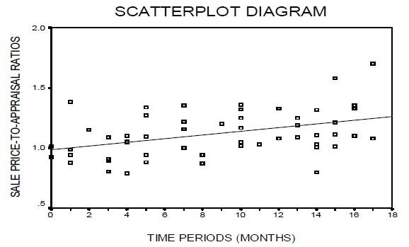
| No. of Observations | 54 |
|---|---|
| Sig T | 0.001 |
| Constant | 0.984 |
| X Coefficient | 0.0015 |
| No. of Observations = | The number of rows of data being analyzed in the data set |
|---|---|
| Sig T = | The significance of T statistic provides a measure of certainty as to whether the trend is valid and should be considered |
| Constant = | The y-axis intercept |
| X Coefficient = | The slope for each independent variable |
The Sig T Statistic is a statistical test that is used to evaluate the significance of a hypothesis. The hypothesis in time trending is that there is not a time trend. If the Sig T Statistic is less than 0.05, then the hypothesis is rejected and the time trend is deemed statistically significant. In other words, the appraiser can be ninety-five percent confident that a time trend should be applied. If the Sig T Statistic is between 0.05 and 0.10, the time trend is deemed “borderline” significant and other direct and indirect time trending techniques should be examined before deciding whether to apply a time trend adjustment. If the Sig T Statistic is greater than 0.10, the time trend is deemed insignificant and should not be applied.
The sales ratio trend analysis in the example utilizes non-weighted least squares regression of the base year S/A ratios over time. The regression formula calculates a mathematical trend from the ratios that is visually represented in the scatter plot diagram. Measurement of the degree of slope in the trend allows the calculation of the percentage rate of change per month or “time trend”. Since the Sig T is less than 0.05 for the property subclass, the time trend is deemed statistically significant and should be considered.
Calculation of rate of change is determined by applying the following formula:
X Coefficient (Slope) / Constant (Y Axis Intercept)
The resulting number is the rate of change per month (in decimal form) that can be used to time trend sales prices to the appraisal date.
Calculation of the time trend for the example data set is shown below:
X Coefficient / Constant = Rate of Change per Month
0.015 / 0.984 = 0.0152 or 1.52 percent increase per month
Advantages of Sales Ratio Trend Analysis
- There is less concern with stratification by property characteristics. A sales ratio reflects the relationship between the sales price and the value that exists for properties of different physical characteristics. However, stratification and analysis by subclass and location should be performed to determine if different time trends exist.
- Nonlinear (curved) rates of change can be determined using sales ratio trending. However, the methods used to determine and measure nonlinear rates of change are more complex than described here.
- Sales ratio trending is easily administered as a component of any sales confirmation program. The only data required are the previous value, sales price and sale date.
- Time trending factors determined from other trending techniques can be compared and analyzed to determine if the effect of time is accurately represented.
Disadvantages of Sales Ratio Trend Analysis
- The assessor's actual value for each sale must reflect the property characteristics for which the sales price was established.
- Another limitation to sales ratio trend analysis is the assumption that the previous year’s values reflect correct market values of the previous appraisal date.
- The distribution of sales ratios used in this analysis must be representative of properties within the analysis area. Additional analysis should be performed to ascertain the representativeness of the sales ratio trend analysis sample.
As a reminder, sales ratios used in the sales ratio analysis technique must be based on the existing actual values that have been determined for the prior general reappraisal cycle. For the reappraisal year, sales ratios should be calculated using the sales prices collected during the data collection period ending June 30 of the prior year, divided by the assessor's actual values reflecting the prior base period appraisal date.
Multiple Regression Analysis
Multiple regression analysis (MRA) is a technique for determining the influence of several independent factors, called independent variables, on a single dependent variable, usually the total market value of the property. Examples of independent variables are size in square feet, location, age, and other property characteristics.
If time of sale is one of the independent variables, its effect on market value can be estimated and an average rate of change in price levels can be extracted. For example consider the following MRA derived model.
MV (Market Value) = $10,909.93 + ($499.78 X months since sale) + ($43.10 X sq.ft.) + ($121.90 X location) + etc.
Here the independent variables include:
- Number of months since the sale occurred to the appraisal date (months since sale)
- Square footage of the property (sq.ft.)
- Location of the property (location) as a dummy variable
Each of these independent variables has a multiplier, called a coefficient. If the regression analysis determines a coefficient for number of months since sale of $499 and the average sale price is $100,000, then the average indicated rate of change is approximately 0.005 percent per month ($499 ÷ $100,000) or 6 percent per year (0.005 X 12).
It must be emphasized that this is simply an average indicated rate of change and that the actual rate of change in this model would vary from property to property depending upon the property's sale price or calculated market value. Also, this is a linear model in that every additional month from the appraisal date would add $499 to the calculated value.
More realistically, multiple regression can be used to develop nonlinear (curved) adjustments for time. And to improve accuracy of the resulting calculated market values, separate regression models can be built for different stratifications of property.
Development of MRA models is beyond the scope of these procedures. Please refer to Property Appraisal and Assessment Administration, IAAO, (1990) for additional information on MRA model building. Also recommended are IAAO Course 311 – Residential Modeling Concepts and Course 320 - Multiple Regression Analysis.
Advantages of MRA
- Regression allows for analysis of large amounts of data.
- This technique can easily manipulate data to test theories and hypotheses.
- Contributory values for many property characteristics can be tested. Those property characteristics that significantly influence value can be identified and their influence on value can be statistically verified.
- MRA can include nonlinear (curved) relationships within and between property characteristics.
Disadvantages of MRA
- MRA may produce unreliable results with small sample sizes.
- The technique is difficult to explain to taxpayers.
- To properly use all aspects of the technique requires knowledge of statistics.
- Time trends are not "decomposable", i.e., they cannot be separated from their interaction with other variables. Time trends extracted from MRA are best used as a comparison to trends developed from other time trend techniques and should not be exclusively applied outside the regression equation.
Application of Time Adjustments
Application of monthly time adjustments to sold property prices for paired sales, property resales, and sales ratio trend analysis determined monthly time adjustments are to be applied as shown in the following example.
Time adjustments should be applied to all confirmed sales using the following formula.
TASP = SP[1 + (rt)]
TASP = Time Adjusted Sales Price
SP = Sales Price
r = Time adjustment percentage decimal equivalent. This will be a negative number in a declining market.
T represents the number of months between the month of sale and the June 30th appraisal date.
In using the time adjustment technique, the assessor should be aware of the following:
- To achieve an accurate time adjustment estimate, all sales must be confirmed.
- When using two or more sales of the same property to establish time adjustments, the property must not have had any material physical change between dates of sale.
- All sale dates should be identified as occurring in the same month that the transaction occurred.
- All sales should be inspected at the time of sale to ascertain their physical characteristics.
As soon as confirmed land sales are adjusted for time, they should be plotted on land maps. Ideally, these maps would be the same maps on which zoning (land use) and economic area boundaries have been drawn. Assessors may prefer, however, to post land use and economic area boundaries on base maps and to post sales data on individual property maps that show land dimensions, shape and size.
Both the time adjusted sales price and the price per unit should be shown within the boundaries of the land sold. A standard unit price can then be developed for each street or block and shown on the land valuations map. This permits the assessor to note the location of sales and to detect price per unit patterns.
Information on making time adjustments can be found in the following publications:
- Property Appraisal and Assessment Administration, 1990, International Association of Assessing Officers.
- Property Assessment Valuation, 2010, International Association of Assessing Officers.
- Fundamentals of Mass Appraisal, 2011, International Association of Assessing Officers.
Adjustments for Differing Property Characteristics
Location Adjustments
Assuming economic areas have been properly determined, few location adjustments will be needed. If a large number of properties within an economic area need individual location adjustments, redefining the economic area boundaries may eliminate some or most of these adjustments. Economic area boundaries can be changed if they are in error or when the change is justified by economic forces and factors.
If there is a lack of economic area sales, it may be necessary to use sales from other economic areas. If additional sales are needed, the objective is to find two or more similar properties where the only difference is economic area location. Once the difference has been analyzed and converted to a dollar or percentage adjustment, this adjustment may be applied to all similar sales used from the other economic area.
Information on making locational adjustments can be found in the following publications:
- Property Appraisal and Assessment Administration, 1990, International Association of Assessing Officers.
- Property Assessment Valuation, Third Edition, 2010, International Association of Assessing Officers.
Other Physical Characteristics Adjustments
Adjustments for access, view, topography, soil types, and many other possible physical differences are included in the physical characteristic adjustment process. Like locational adjustments, some other physical characteristic adjustments can be eliminated if initial economic area boundaries are properly defined. Economic area boundaries can be changed when the change is justified by economic forces and factors.
The adjustment for physical characteristics also includes analysis and adjustment for size, shape, and corner location characteristics that may not be representative of the typical parcel under appraisal. These characteristics and influences include the following:
- Corner influence
- Depth influence
- Surplus land influence
- Irregular sizes and shapes influence
Corner Influence Adjustments
Corner influence is the degree by which land value changes for a corner lot compared to the value of an otherwise comparable inside lot. In the case of business property, the added usefulness and value of corner lots results from the accessibility of two or more streams of pedestrian traffic, additional window displays, more prominence, and availability of more light and air than inside lots.
In the past, corner influence rules or tables have been used by assessors as a guide in mass appraisal work, especially in primary and secondary retail business districts. In practice, however, these rules and tables were found not to be representative of changing market conditions. Using the values derived through such formulas alone can lead to unsound value estimates.
In some residential areas, corner lots may command lower prices than inside lots of comparable size and characteristics. The corner influence may actually be a negative factor due to the possibility of greater special assessments, lack of privacy, increased noise and dirt, added care of curb and sidewalks, and reduction in lot area by building set-back requirements for each street.
In other residential subdivisions, corner influence may be a positive factor. A corner lot may bring a premium due to the fact that a house may be faced in either of two directions or placed diagonally on the lot allowing a view of both directions and construction of a curved driveway that exits on both streets.
However, no universal rule or table applies and the assessor must look to the market for evidence of the effects of location on value. Local attitudes, land-use patterns, rent levels, and sales prices should be analyzed to find out whether corner influence exists.
When analyzing sales, the assessor should exercise caution when attempting to attribute increases or decreases in sales prices to corner influences. In many cases, the increase or decrease can be attributable to other factors such as general location, or access. In other cases, a corner influence may exist in some parts of the neighborhood, but not in others. A substantial number of sales must be analyzed to ascertain whether a corner influence exists and how much of an adjustment should be made.
For information on corner influence, refer to the following:
- Property Appraisal and Assessment Administration, 1990, International Association of Assessing Officers.
- Property Assessment Valuation, Third Edition, 2010, International Association of Assessing Officers.
Depth Influence Adjustments
Lots in the same economic area can vary in depth, even from one side of the street to the other. Usually, an increase in depth will cause an increase in value. However, the value increase may not be proportionate to the increased depth of the lot. When this is the case, depth factors should be developed as an aid to valuing lots with atypical depths. To account for all likely atypical depths, these factors are usually placed in a depth table for ease of use.
Depth factors can only be developed through an extensive analysis of market sales. It is possible that, depending on individual economic area sales analysis, each economic area could have different depth factors listed in their depth tables.
Depth factors should be used cautiously. Without good judgment they can become crutches to support unrealistic values. All facets of land valuation are based upon analysis of the market in which a particular property is located and the use of any table must be consistent with the conditions of that market.
For specific information on development of a depth table, refer to the following.
- Property Appraisal and Assessment Administration, International Association of Assessing Officers, 1990.
- Property Assessment Valuation, International Association of Assessing Officers, 2010.
Surplus Land Influence Adjustments
Any parcel of land containing one building site that has more land than is necessary for a typical building site, but cannot be separated from the site and does not have an independent highest and best use, is deemed to have surplus land. Because of the surplus land, application of a square foot or front foot unit of comparison to the entire parcel would likely result in an erroneous value. An erroneous value exists either because as land size increases beyond what is typical for a building site, people will not pay for the added amount of land at the same rate as they would pay for a typical building site, i.e., the added land does not have the same degree of utility to the prospective buyer as the typical building site; or, in the case of frontage value, the established value of a front foot does not account for the marginal increase or decrease in value due to excess land.
Surplus land may be found in residential and commercial property. An example of surplus land influence calculation is shown below.
Example:
You have confirmed several residential land parcel sales, each containing approximately 25,000 square feet at a sale price of $3,750 or $0.15 per square foot for each site. From other existing sales you determine that a typical residential building site within the neighborhood is 15,000 square feet and sells for $0.20 per square foot. What would be a reasonable estimate for surplus land adjustment and what value would you place on a parcel of 20,000 square feet?
Surplus Land Influence Calculation
| Sales Price | Parcel Size | SP per sq ft | |
|---|---|---|---|
| Oversize lot | $3,750 | 25,000 | $0.15 |
| Typical lot | -$3,000 | -15,000 | $0.20 |
| $750 | 10,000 |
Note: Sales Price attributable to surplus land ($750 ÷ 10,000 sq. ft.) = $0.075
Valuation of subject lot (20,000 sq. ft.)
| Typical site | 15,000 sq. ft. x $0.20/sq. ft. = | $3,000 |
|---|---|---|
| Surplus land | 5,000 sq. ft. x $0.075/sq. ft. = | $375 |
| Subject lot value 20,000 sq. ft. = | $3,375 |
Surplus land influence can differ greatly by economic area location. A surplus land adjustment for one economic area may not work for other economic areas. If possible, surplus land adjustments should be determined for each economic area.
Be aware that land adjustments can increase greatly if the additional land area can be separated and built on while conforming to local zoning and building codes.
Irregular Size and Shape Influence Adjustments
There are other adjustments that can be made for atypical lot sizes and irregularly shaped lots. However, these adjustments are seldom used in Colorado. If the economic area under appraisal has a substantial number of lots with varying sizes and shapes, it might be prudent to review the unit of comparison used to value the lots.
In most cases, converting to a building site or units buildable unit of comparison would allow for consideration of the atypical sizes and shapes without requiring the appraiser to spend time developing special modifiers that may be useful in only a few cases.
For information about unit modifiers for size and shape adjustments, please refer to the following:
Property Appraisal and Assessment Administration, International Association of Assessing Officers, 1990.
Calculation of Adjustment Amounts
Calculation of Adjustment Amounts Using Matched Pair Analysis
Adjustment amounts are generally determined by "matched pair" analysis of time-adjusted comparable sales. Closely comparable sales are listed in groups of two, sales prices are analyzed, and the differences in sales price between the two sales are attributable to differences in location or physical characteristics between the properties.
This process works only if the time adjusted sales are virtually identical properties except for one difference in physical characteristic or only a difference in location.
An example of this calculation is shown below.
Example:
In your sales confirmation program, you have confirmed two land sales for identical properties except for view. Sale #1 is a generally flat, residential lot with an average view of the mountains that sold for $5,000. Sale #2 is a generally flat residential lot that does not have a view of the mountains that sold for $4,500. Each lot contains one building site and both are considered a typical size for the area. All sales have been previously time adjusted.
| Sale #1 (with view) | $5,000 |
|---|---|
| Sale #2 (no view) | 4,500 |
| Sales Price attributable to view amenity | 500 |
Percentage adjustment determination
$5,000 ÷ $4,500 = 111%; difference is 11%
If a subject property or properties has a mountain view, all sales without a mountain view should be adjusted +11 percent if they are to be used to value the subject property.
Calculation of Adjustment Amounts Using Cost to Cure
Occasionally, physical differences between comparable sales and the subject property can be determined by using the cost to cure method. Using an existing cost manual, cost valuation service, or other source of construction costs, the assessor can estimate what cost would be necessary to adjust for the differences between the comparable sale(s) and the subject.
Obviously, this method cannot be used for adjustments of an intangible nature or that are not feasible to cure. Examples of this type of intangible or non-feasible adjustment would be as follows:
- View
- Location
- Topography
- Soil Conditions
- Other intangible adjustments or adjustments that cannot economically be cured
An example of a cost to cure adjustment calculation technique can be found below.
Example:
You are trying to determine an adjustment amount for lots that have a summer use only dirt road for access. You have gathered and confirmed sales of two lots that are similar to the subject lots in every way except they have gravel, all weather roads for access. The length of the access road for both the subject and the comparable is approximately 100 feet. The access road for both sales is new. You were unable to confirm any other sales of lots that had the same access problems as the subject.
Sale #1 sold for $10,000 and Sale #2 sold for $9,800. All sales have been time adjusted to the end of the data collection period.
Using your cost service manual, you determine the following linear foot cost for grading a 12' road and adding a 3" rock gravel road base similar to the road to each of the comparable properties.
| Cost of Grading to upgrade road: | $4.60 per linear foot |
|---|---|
| Add 3" Gravel road base: | $10.00 per linear foot |
| $14.60 per linear foot |
To adjust the comparable sale to account for the lack of an all-weather access road, you would deduct the replacement cost of the road from the sales price paid for each of comparable lot sales.
Sale #1: $10,000 - 1,460 = $8,540
Sale #2: $9,800 - 1,460 = $8,340
Caution should be exercised when using this cost adjustment technique. When applied properly, the cost approach usually generates the upper limit of value for property valuation. Because of economic conditions within the economic area, the market may determine that the contributory value of the improvement is less than its cost. This method should be used only when no market information is available.
Calculation of Adjustment Amounts from Other Sources
When the matched pair and cost to cure methods cannot be used because of insufficient information, the assessor must use other sources of information. However, confirmation of sales from the full five-year data collection period should occur before consideration of other sources.
One other source would be sales from other counties having similar economic conditions. If local sales are absent, sales from economically comparable counties are a good source.
Another less reliable source, to be used only as a last resort, is the soliciting of opinions from local appraisers and real estate professionals concerning the contributory values of characteristics for which adjustments are necessary.
Comparable Sale Adjustment Techniques
Adjustments to comparable land sales can be made in one of three ways:
- Adding and subtracting dollar amounts
- Adding or subtracting percentage adjustments
- Cumulative multiplication of percentages
Examples of each of these adjustment techniques are shown below.
Example: Addition/Subtraction of Dollar Adjustments
| Sales Price | $16,000 |
|---|---|
| Plus Adj for Time (+5 percent) | + 800 |
| Time Adjusted Sales Price | $16,800 |
| Plus Adj for View (+10 percent) | +1,680 |
| Plus Adj for Location (+5 percent) | +840 |
| Less Adj for Access (-5 percent) | -840 |
| Total Adjustment | +1,680 |
| Adjusted Sales Price | $18,480 |
Example: Addition/Subtraction of Percentage Adjustments
| Sales Price | $16,000 |
|---|---|
| Plus Adj for Time | x 1.05 |
| Time Adjusted Sales Price | $16,800 |
| Plus Adj for View | + 10% |
| Plus Adj for Location | + 5% |
| Less Adj for Access (-5 percent) | - 5% |
| Total Adjustment Percent | +10% |
| Adj Sales Price ($16,800 x 1.10) | $18,480 |
Example: Cumulative Multiplication of Percentage Adjustments
| Sales Price | $16,000 |
|---|---|
| Plus Adj for Time | x 1.05 |
| Time Adjusted Sales Price | $16,800 |
| Plus Adj for View | x 1.10 |
| Plus Adj for Location | x 1.05 |
| Less Adj for Access | x 0.95 |
| Total Adjustment Percent | 1.097 |
| Adj Sales Price ($16,800 x 1.097) | $18,430 |
A slightly different value may result from addition and subtraction versus multiplication of percentages, but the difference is usually not sufficient to materially affect the final valuation.
An example of the adjustment process, using both percentage and dollar amount adjustments, is shown below.
You are appraising a residential lot in a mountain subdivision. The subject property contains 2.2 acres and has an excellent view. The topography of the lot indicates steep terrain with poor access because the roads are not in good repair. The lot does not have a water well.
The appraisal date is June 30th of the year preceding the year of general reappraisal.
The following comparable sales have been confirmed as qualified sales:
Sale #1: Located in a flat part of the subdivision, this property has average view and good access. It sold ten days ago for $11,400. There is no water well on the property.
Sale #2: Located in a steep part of the subdivision, this property has average view and poor access. It sold about one year ago for $9,800. There is no water well on the property.
Sale #3: Located in a steep part of the subdivision next to the subject property, this property has excellent view and poor access. It sold about one year ago for $17,000. There is a water well on this property.
All lots are about 2 acres, wooded and all have underground electric service. All lots have access to water if wells were drilled. Only a few lots have wells at this time.
The following market factors have been determined from the market:
Time Adjustment – 5 percent increase per year.
Other Adjustments – As determined from market analysis of sales within the subdivision:
Lots with excellent view sell for $2,000 more than lots with average view.
Steep lots sell for $500 less than flat lots.
Lots with poor access will sell for $500 less than lots with good access.
A well will add $6,000 to the value of any lot.
When adjustments are made to the comparable sales prices to make them similar to the subject property, an adjustment grid is generated as shown below
Example:
| Subject | Sale #1 | Sale #2 | Sale #3 |
|---|---|---|---|
| Sales Price | $11,400 | $9,800 | $17,000 |
| Time Adj. | x 1.05 | x 1.05 | |
| Time Adj. S.P. | $11,400 | $10,290 | $17,850 |
| View excellent | + 2,000 | + 2,000 | |
| Access poor | - 500 | ||
| Terrain steep | - 500 | ||
| Well none | -6,000 | ||
| Total Adj. | + 1,000 | + 2,000 | -6,000 |
| Adj. S.P. | $12,400 | $12,290 | $11,850 |
Generally accepted appraisal theory indicates that the most reliance should be placed on the comparable sale or sales that are the most similar to the subject property and have the least adjustments. All three of the adjusted comparable sales indicate relatively tight adjusted sales price range of $12,400 to $11,850. Sale #3, by virtue of its similarity of view, access, terrain, and location next to the subject, would have the most reliance placed upon it. Therefore, the assessor’s estimate of value for the subject parcel would be approximately $12,000.
For more information on adjustment techniques, please refer to Property Appraisal and Assessment Administration, 1990, International Association of Assessing Officers.
Comparable Sales Analysis Process – Final Estimate of Value
The amount remaining after all adjustments to vacant land have been made is termed Adjusted Selling Price (ASP). If present worth valuation procedures are applicable to the property, then these additional procedures must be applied. Specific information about present worth procedures is located in Chapter 4, Valuation of Vacant Land Present Worth, later in this manual.
If present worth valuation procedures are not applicable to the property, then the comparable sales need to be reviewed, adjusted, and reconciled into a final estimate of value.
In the reconciliation process, the greatest weight is given to those sales that are the most comparable to the subject property and have the least number of adjustments. Sales that require a large number of adjustments are given less weight. If, after comprehensive analysis, all comparable sales are determined to have equal weight, the midpoint of the adjusted selling price value indications should be used.
Extraction and Allocation Methods
The extraction and allocation methods are variations of the market approach to valuation. These methods require the use of a sufficient number of recent sales to establish a trend or pattern for allocation or extraction of land values from aggregate property values.
Extraction Method
The extraction method involves determination of the contributory value of the improvements as part of the total sales price of an improved property. The balance of the sales price is attributed to the land.
When a particular area has been fully developed and there are no recent sales of vacant lots, the assessor may either apply land values established by comparable sales in very similar economic areas or may extract the value of the land from current improved property sales within the economic area. The extraction procedure involves inspection, listing, and grading the quality of the improvements and applying the appropriate cost and depreciation schedules to arrive at the depreciated value of the structure at the date of sale.
By deducting the depreciated value of the improvements from the sales price of the entire property, the assessor can obtain the extracted value of the land.
Example:
| Time Adjusted Sales Price | $45,750 |
|---|---|
| Market Value of Comparable Improvements | $36,750 |
| Extracted Land Value | $9,000 |
Example:
| Time Adjusted Sales Price | $45,750 |
|---|---|
| Replacement Cost New | $52,500 |
| Depreciation - 30% | -$15,750 |
| RCNLD | $36,750 |
| Extracted Land Value | $9,000 |
This method must be used with caution. The accuracy of the land value indicated by the use of this method depends largely on the reliability of the market value of comparable improvements. Very small errors in estimated improvement values can result in large errors in the remaining value, i.e., in the extracted value of the land. In addition, the subject land parcels and the improved properties ideally should be located in the same economic area and must have the same use.
Allocation Method
Under the allocation method, a portion of total property value is assigned to the land. Relationships between land and improvement are usually determined from the following sources:
- Site values in previous years
- Land-to-building ratios in similar neighborhoods
- Analysis of new construction on similarly classified sites
Example:
You are appraising land in a neighborhood where there are no vacant land sales. Research in residential neighborhoods similar to that of the subject property indicates that a typical land to building ratio should be about 1:4 (one part land to four parts building). Consider then, that the land is one part of the five total parts. The typical improved property sale in this neighborhood is $40,000.
Allocation of value to the land should be 1/5 or 20 percent
$40,000 x 0.20 = $8,000 Indicated land value.
Caution also must be exercised when using this method. There must be a high degree of comparability among the sites and among the properties. The properties must be located in the same economic area and be subject to the same market influences. While this method is simple, it involves several subjective assumptions and can result in an uneven pattern of land values.
Anticipated Use or Developmental Cost Method
The cost approach is generally not applicable to land valuation due to the following reasons:
- Land is a finite commodity and no replacement cost can be established for it.
- Land does not depreciate.
However, in valuing subdivisions and land developments, the cost approach may be used in estimating the value of site improvements. The anticipated use or developmental cost method, requires the appraiser to estimate the highest and best use of a tract of raw land and then to hypothetically develop the site. From the total projected sales prices of the developed lots, all costs of development are subtracted. The resulting residual value indicates the value of the raw land. Usually, the total residual value is divided by the total number of acres to get the raw land value per acre.
Site development costs include costs of utilities, streets, curb and gutter and other site improvements. These costs, along with the raw land cost (sales price) are added together to determine the total land development cost. The assessor should obtain both the raw land and site development costs from typical subdividers and land developers within the county.
Land that is changing use between raw land and the highest and best use as residential or commercial tracts can be valued using the anticipated use or developmental cost method.
In using this method, caution should be exercised for the following reasons:
- This method is highly theoretical and requires a number of estimates regarding gross lot sales revenue, sellout period, development costs, and site layout.
- The analysis required is complicated and an assumption must be made that the land’s highest and best use is for subdivision development.
- The sales of all of the lots may not be realized within one year. If a sell-out period of several years is anticipated, the sales prices likely will have to be discounted to present value using Column #5 of the compound interest tables.
- Development costs will have to be researched by the appraiser. This research may be difficult and may take a substantial amount of time to complete.
This method should only be used when comparable sales are not available.
Specific information about the anticipated use and development method can be found in the following publications.
- Property Appraisal and Assessment Administration, 1990, International Association of Assessing Officers.
- Encyclopedia of Real Estate Appraising-3rd Edition, 1978, Friedman, Edith, General Editor, Prentice-Hall Inc, Englewood Cliffs, N.J.
- Property Assessment Valuation, 2010, International Association of Assessing Officers.
Capitalization of Ground Rent Method
A useful methodology for land valuation by the income approach is the capitalization of ground rent method.
This method is based on the premise that value is determined by the present worth of future benefits of property ownership. The market rent of the subject site is estimated, a net income is calculated, and a capitalization rate selected. The net income is then capitalized into an indication of value by dividing the net income by the capitalization rate. The capitalization rate can be developed by either a market study, the band of investment method, or the summation method.
A market capitalization rate is developed through analysis of land sales that have a typical net operating income stream. Dividing the annual net operating income by the confirmed sale price results in a capitalization rate. Review of all the resulting market capitalization rates will allow the assessor to determine the rate that best fits market conditions within the county.
For the purposes of demonstration, assume that comparable rental data indicate that a subject site would rent or lease for a net operating income of $1,000 per year. A market study indicates that the proper land capitalization rate is 10 percent. The net operating income would be capitalized into value as follows:
$1,000 ÷ 10% = $10,000
Example:
A retail building is located on leased land. The land parcel is 15,000 sq. ft. and rents for $0.50 net per sq. ft. per year. Market research indicates that the economic capitalization rate is 12.5 percent.
15,000 sq. ft. x $0.50/sq. ft. = $7,500 Net Annual Rent
$7,500 ÷ 0.125 cap rate = $60,000 Indicated Land Value
Development of a capitalization rate using the band of investment method requires knowledge of the total sales price of a property, the percentage of the sales price attributable to the owner’s equity interest, the owner’s equity yield requirements and the percentages and interest rates associated with mortgage financing of the property. Using this information, a band of investment capitalization rate is determined, as shown in the following example.
Example:
| Yield or Interest | Percent of Total Capital |
|---|---|
| First Mortgage 15% (0.15) | X 55% (0.55) = 0.0825 |
| Owner’s Equity 13% (0.13) | X 25% (0.25) = 0.0325 |
| Second Mortgage 18% (0.18) | X 20% (0.20) = 0.0360 |
| Band of Investment Capitalization Rate | 100% = 0.1510 |
Summation
Development of a capitalization rate using the summation method requires the assessor to determine rate components for the safe rate, the management rate, the risk rate, and consideration for illiquidity. This method should only be used when there is a lack of market sales of comparable properties. It requires the assessor to make several subjective judgments regarding management, liquidity, and risk rate components. The summation method is described in detail in Chapter 4, Valuation of Vacant Land Present Worth.
The capitalization of ground rent method is also feasible when land is rented or leased independently of improvements. There are many instances in which commercial land is leased on a net basis. Care should be exercised to determine whether any long-term leases reflect current economic rents.
In cases where commercial land is leased on a short-term basis (one to ten years), the net rent can be directly capitalized into an indication of land value.
Residual (Land) Method
Another capitalization of income approach method is the land residual method. However, the land residual method can only be used when a building is proposed or when the existing building does not suffer from physical deterioration or functional or economic obsolescence. Therefore, this method should only be used as a last resort.
This method requires that the highest and best use of the property be estimated. The net income from the total property is estimated from comparative market income data. The replacement cost new of a building is estimated and income attributable to the building determined by multiplying the building value by the building capitalization rate. This income is then deducted from the total net income. The remaining income is attributable to the land and is capitalized into an indication of value by dividing the remaining income, i.e., the income attributable to the land, by the land capitalization rate.
Example:
You are appraising the land under a new office building. The building has a replacement cost new of $165,000 and a remaining economic life of 50 years. Economic net income to the property is $30,000. The building has not suffered any form of depreciation.
The applicable discount rate, developed from a market study is 9.5 percent. The local mill levy is 90 mills and the assessment rate is 29 percent. Calculate the land value by the land residual method.
| Discount rate | 9.5% (developed from market study) |
|---|---|
| Effective Tax rate | + 2.6% (0.29 assessment rate x 90 mills or 0.09) |
| Land Cap Rate | 12.1% Rounded 12% |
Discount/Tax rate (Land capitalization rate) = 0.12
Building recapture rate (1÷50)= 0.02
Building capitalization rate = 0.14
| Building value: | $ 165,000 |
|---|---|
| Building cap rate: | x 0.14 |
| Income attributable to building | $ 23,100 |
| Total net income | $ 30,000 |
|---|---|
| Building net income | - 23,100 |
| Land net income | $ 6,900 |
| Land net income | $ 6,900 |
|---|---|
| Land cap rate | ÷ 0.12* |
| Indicated land value | $ 57,500 |
*Land does not depreciate. Therefore, the building recapture rate is not added.
Reconciliation of Land Valuation Approaches
In reconciliation of the value estimates from the applicable valuation methods used to value any property, the appraiser takes into account the reliability of available data along with the purpose of the appraisal. Reliance by the appraiser, within the requirements of the statutes, on the most defensible method should lead to a realistic final estimate of value.
Colorado Statutory and Case Law Requirements
Colorado statutes require that the cost, market, and income approaches to value be considered in the valuation of all land except for land used for agricultural and residential purposes, oil and gas leaseholds and lands, and for producing mines. For agricultural land, an approved formula that complies with statutory language and legislative intent is to be used. This formula capitalizes net landlord income into an indication of value. For residential improved property, only the market approach is to be used. For oil and gas leaseholds and lands and producing mines, statutory formulas are used.
In determining which valuation approach or approaches should be used, Colorado case law, Montrose Properties, LTD., et al., v. Colorado Board of Assessment Appeals, et al., 738 P.2d 396 (Colo. App. 1987), affirms that the assessor must give appropriate consideration to all required approaches to value. In this case, the court concluded that “appropriate consideration” was used by an assessor when the assessor decided that insufficient information precluded the use and calculation of one or more of the required approaches. The court reasoned that appropriate consideration was used in determining that the approach(es) was not applicable. The need for appropriate consideration of the three approaches was also affirmed by the Colorado Supreme Court in Board of Assessment Appeals, et al., v. E.E. Sonnenberg & Sons, Inc., 797 P.2d 27 (Colo. 1990).
Realistically, unless sufficient income information exists for the use of the income approach, the market approach generally should be the basis for the final land valuation. To apply the market approach in the valuation of vacant land, the appraiser should be familiar with Chapter 4, Valuation of Vacant Land Present Worth. Documentation of the market approach and documentation of the non-applicability of the other approaches should be developed to satisfy the requirements of the § 39-1-103(5), C.R.S.
Information Access and Confidentiality
At the written request of any taxpayer or taxpayer’s agent, and subject to such confidentiality requirements as provided by §§ 24-72-204 and 39-5-121.5, C.R.S., the assessor must make available the data used in determining the actual value of any property owned by the taxpayer within seven (7) working days following the written request. Upon receiving the request, the assessor must immediately advise the taxpayer or agent of the estimated cost of providing the data. The intent of the statute is that the assessor immediately estimates the cost because payment must be sent to the assessor prior to providing the data. Once the data is gathered, the assessor can choose whether the data is mailed, faxed, or sent by electronic transmission to the taxpayer or agent. If the estimated cost was lower than actual costs, the assessor may include a bill with the data for any reasonable cost above the estimated cost subject to the statutory maximum. The additional costs are due and payable upon receipt of the data.
Such confidential information would include sales information obtained from the Real Property Transfer Declaration (TD-1000), the “Manufactured Home Transfer Declaration,” or other supplementary sales confirmation documents. However, the data from these documents can be combined and summarized so that individual properties or owners are not identified. These summaries can then be made available to the taxpayer as required by § 39-5-121.5, C.R.S.
It is further suggested that summaries of confidential income data for the various economic areas in the county be prepared. For example, a summary of economic area #1 would reflect gross rents ranging from $X to $Y and expenses ranging from $A to $B, etc. It is important that the assessor ensure confidentiality in all cases.
If a Computer-Assisted Mass Appraisal (CAMA) process is used to determine values, any nonproprietary data used to create the valuation model must also be made available for review by the taxpayer.
This data should be made ready for distribution prior to the taxpayer protest period. This will allow ample time to delete confidential source notations yet supply all information to which the taxpayer is entitled.
Pursuant to § 24-72-205, C.R.S., the statutory maximum is $0.25 per page unless actual costs exceed this amount. The statute delineates how the charges may be calculated. For additional information regarding this issue, refer to ARL Volume 2, Administrative and Assessment Procedures, in Chapter 1, Overview of Assessor’s Duties and Relationships.
Reference Sources for Land Valuation
Additional information about land valuation techniques, appropriate units of comparison, adjustments to sales, and other information may be obtained by consulting the following publications:
- Property Appraisal and Assessment Administration, 1990, International Association of Assessing Officers, 314 West 10th St., Kansas City, MO 64105-1616.
- The Appraisal of Real Estate, 2013, 14th Edition, Appraisal Institute, 550 West Van Buren, Chicago, Illinois 60607.
- Fundamentals of Mass Appraisal, 2011, International Association of Assessing Officers, 314 West 10th St., Kansas City, MO 64105-1616.
- Standard on Ratio Studies, 2010, International Association of Assessing Officers, 314 West 10th St., Kansas City, MO 64105-1616.
- Property Assessment Valuation, 2010, 3rd Edition, International Association of Assessing Officers, 314 West 10th St., Kansas City, MO 64105-1616.
- Improving Real Property Assessment, 1978, A Reference Manual, previously published by the International Association of Assessing Officers, 314 West 10th St., Kansas City, MO 64105-1616.
- Mini-Math for Appraisers, 1974, Irvin E. Johnson, previously published by the International Association of Assessing Officers, 314 West 10th St., Kansas City, MO 64105-1616.