Statistical Performance Analysis
The beginning, intermediate, and final step in ad valorem appraisal is to conduct statistical performance analyses. These analyses use descriptive statistics to measure central tendency and to measure the relative variability of data about the measure of central tendency. These measures are then compared to the acceptable measurement ranges for statistical compliance established by the State Board of Equalization (state board). Assuming the statistical sample size is adequate, measures that fall outside the acceptable ranges indicate that additional appraisal work is needed to discover what has caused outlier values to occur.
It is recommended that preliminary statistical analysis be completed before the initial reappraisal plan is developed. This analysis can identify property classes, subclasses, economic areas, and other property strata, e.g., price range, size, age, quality, condition, and design, most in need of appraisal attention. Statistical analysis is also the final step in ensuring the overall accuracy of reappraised values. Statistical analysis is a measurement of the success of a reappraisal.
In evaluating vacant land, residential improved, and commercial/industrial improved classified property values in Colorado, the following measures frequently are used:
- Measures of Central Tendency
- Median assessment ratio (primary measurement)
- Mean assessment ratio
- Weighted mean assessment ratio
- Measures of Relative Variability
- Coefficient of dispersion (primary measurement)
- Standard deviation
- Coefficient of variation
- Measure of Assessment Bias
- Price related differential (primary measurement)
- Measure of Confidence in Statistical Results
- Confidence interval
Sampling Techniques and Sample Size
A sample is a data set drawn from a population. Most market analysis and statistical analysis procedures rely on sampling because of the time and expense attempting to obtain data on all items in the population. If the sample is properly drawn and it represents the population, sampling can be a reliable market and statistical analysis tool.
Two basic types of sampling are probability sampling and nonprobability sampling. Probability sampling is one in which every item in the population has an equal chance of being selected. Probability sampling includes random, systematic, stratified, and cluster sampling techniques. For the most part, assessors will use random and stratified sampling in determining market and statistical analyses.
Selecting a random sample involves assigning every element in the population a number and choosing the sample by using a random number table generated either by computer or contained in a random number book.
For example, an assessor wants to determine if a complete physical inspection of every residential property is necessary to properly value all residential property in the county. The assessor should develop a random sample of properties on which to make a personal field inspection to compare existing property inventories with what is actually in place. Depending on the number of mistakes and omissions that exist, the assessor may determine that a complete physical inspection is necessary or only a cursory drive-by review can suffice.
Stratified samples are gathered from a population that is stratified by some characteristic and each stratum is randomly sampled.
A nonprobability sample is one in which not every item of the population has an equal chance of being included. Examples of nonprobability samples include quota and judgment samples. Nonprobability sampling techniques are most commonly used in advertising and business economics decision making. Nonprobability sampling is not recommended in ad valorem work.
Two limitations of sampling are sampling error and bias.
Sampling error is a relative measure, determined by a probability analysis, that the sample is not representative of the population. A sample must be drawn and weighted so that the characteristics of the sample represent or "mirror" the characteristics of the population as close as possible. For example, one area of the county has 60% of the residential improved sales, but only 25% of the population of residential improved parcels. If an assessor were to rely on paired sales in this area only to determine a time trend analysis applicable to the entire county, the resulting time trend factor might be nonrepresentative of the effect of time on all residential properties in the county.
Bias is the incorrect estimation of population characteristics from a poorly designed or executed sample. For example, a county mails an income questionnaire to all commercial businesses in order to ascertain market lease rates. Even though only 10% of the commercial property owners return the questionnaire, the assessor uses this data to determine income values for all commercial property in the county. Bias can exist because of the possibility of only property owners that charge low lease rates returned the questionnaire.
Another possibility of bias results from the failure of the designer of the sample selection technique to provide that every property in the population has an equal chance of appearing in the sample.
For example, an assessor mails out income questionnaires only to his friends and people that have indicated they would fill them out. Although the questionnaire return rate would be very high, the sample likely would be biased because not all commercial property owners would be provided the opportunity to respond.
A properly designed and completed random sample is one of the best ways of ensuring equal representation in the sample of population characteristics. Sample size generally depends on two factors:
- The economic value obtained in the sample
- The cost of sampling
Sample size estimation techniques such as sample mean, standard error of the mean, and standard error of the proportion are all used to determine appropriate sample sizes depending on the desired level of accuracy. However, these techniques are beyond the scope of this section. Please refer to a basic statistics text for additional information on these techniques.
As a general rule for property valuation analysis, the sample size should be sufficient so that the sample is representative of all major value influences affecting the property. Section 39-1- 103(8), C.R.S., details specific sample size limitations and requirements for sales ratio analysis and market analysis for property tax purposes.
Measures of Central Tendency
The three measures of central tendency used in assessment ratio studies are the mean, median and weighted mean. All three measure the tendency of values, i.e., the observed data, to cluster about a central, or representative, value.
Mean
The mean is defined as the arithmetic average of the data elements, e.g., the actual values or sales ratios in a class of property or in a stratification of property. The mean is calculated by adding all of the appropriate values or sales ratios together and then dividing by the number of the data elements summed, i.e., the number of observed ratios.
Median
The median is defined as the value or sales ratio that divides the data elements being analyzed into two halves, with each half containing the same number of observations. It is calculated by listing the data from high to low (or low to high), i.e., arraying the data, and picking the exact middle data element. If there is an even number of data elements (ratios), the median is the average of the two middle data elements.
Weighted Mean
The weighted mean ratio, or aggregate mean ratio, or weighted ratio, is defined as the ratio of the total actual values to the total sales prices in a group. It is calculated by dividing the total actual value of all properties in the subclass or other stratification of properties by the total of the sales prices of those properties. Although a weighted mean could be calculated for any set of data elements, it has been narrowly defined here to apply to ratio studies. The weighted mean measures assessment level on a dollar-by-dollar basis whereas the mean and median do so on a property-by-property basis.
In assessment ratio studies, the median is generally used in measuring assessment level. The median is least affected by a non-normal, i.e., skewed, distribution of data and is least affected by "outlier" data.
Example:
Using the Mean, Median, and Weighted Mean, in Analyzing Typical Commercial Land Sales
| Actual Values | Sales Prices | Ratios* | Arrayed Ratios** |
|---|---|---|---|
| $ 58,900 | $ 65,000 | 0.9062 | 0.7600 |
| 399,500 | 450,000 | 0.8878 | 0.7700 |
| 76,000 | 100,000 | 0.7600 | 0.8067 |
| 742,500 | 750,000 | 0.9900 | 0.8800 |
| 590,000 | 600,000 | 0.9833 | 0.8878 |
| 385,000 | 500,000 | 0.7700 | 0.9062 |
| 800,000 | 800,000 | 1.0000 | 0.9833 |
| 88,000 | 100,000 | 0.8800 | 0.9900 |
| 1,050,000 | 1,000,000 | 1.0500 | 1.0000 |
| 242,000 | 300,000 | 0.8067 | 1.0500 |
| $4,431,900 | $4,665,000 | 9.0340 | 9.0340 |
* Ratio calculated by dividing actual value by sales price.
** All ratios must be arrayed prior to statistical analyses.
Mean Ratio = (9.0340 ÷ 10) = 0.90340 or 90.34%
Median Ratio = (0.8878 + 0.9062) ÷ 2 = 0.8970 or 89.70%
Wtd Mean Ratio = ($4,431,900 ÷ $4,665,000) = 0.9500 or 95%
The state board statistical compliance standards for the level of value for vacant land, residential improved, and commercial/industrial improved classified properties are 95 percent to 105 percent as measured by the median sales ratio.
Measures of Relative Variability
When measures of central tendency are calculated, a single number results. That number represents an entire group of values. However, this number cannot be determined to be truly representative of the group without an indication of the relative distance, or spread, of the data elements from the measure of central tendency. This spread, often called dispersion or variability, is generally measured in assessment ratio studies by the coefficient of dispersion. When using a measure of relative variability, the smaller the coefficient number, the more uniformly assessed are the properties.
Coefficient of Dispersion
Relative variability statistics allow for comparisons within groups of data, such as the ratios which occur when actual values are divided by sales prices.
The coefficient of dispersion (COD) is defined as the measure of the spread of values about the median value. It is calculated by dividing the average absolute deviation from the median by the median. The average absolute deviation is calculated by summing the sign-ignored, i.e., absolute, differences between the median ratio and each of the arrayed ratios and dividing the resulting amount by the number of ratios in the sample being analyzed.
In assessment ratio studies, the COD is generally considered the primary indicator of quality within a mass appraisal project. This is because assessment ratios are not normally distributed. Since there are lower limits beyond which marketplace property values will not fall, the COD is considered more reliable and less prone to the effects of very high (skewed) values often found in property value distributions. In Colorado, the measures of dispersion considered acceptable by the state board are 20.99% or less for vacant land and commercial/industrial improved, and 15.99% or less for residential improved classified properties.
Example:
Using the COD.
| Actual Values | Sales Prices | Ratios* | Arrayed Ratios** | Median Ratio | Absolute Deviation |
|---|---|---|---|---|---|
| $ 58,900 | $ 65,000 | 0.9062 | 0.7600 | 0.8970 | 0.1370 |
| 399,500 | 450,000 | 0.8878 | 0.7700 | 0.8970 | 0.1270 |
| 76,000 | 100,000 | 0.7600 | 0.8067 | 0.8970 | 0.0903 |
| 742,500 | 750,000 | 0.9900 | 0.8800 | 0.8970 | 0.0170 |
| 590,000 | 600,000 | 0.9833 | 0.8878 | 0.8970 | 0.0092 |
| 385,000 | 500,000 | 0.7700 | 0.9062 | 0.8970 | 0.0092 |
| 800,000 | 800,000 | 1.0000 | 0.9833 | 0.8970 | 0.0863 |
| 88,000 | 100,000 | 0.8800 | 0.9900 | 0.8970 | 0.0930 |
| 1,050,000 | 1,000,000 | 1.0500 | 1.0000 | 0.8970 | 0.1030 |
| 242,000 | 300,000 | 0.8067 | 1.0500 | 0.8970 | 0.1530 |
| $4,431,900 | $4,665,000 | 9.0340 | 9.0340 | 0.8250 |
* Ratio calculated by dividing actual value by sales price.
** All ratios must be arrayed prior to statistical analyses.
Median Ratio = 0.8970 or 89.70%
Average Absolute Deviation = (0.8250 ÷ 10) = 0.0825
Coefficient of Dispersion = (0.0825 ÷ 0.8970) = 0.0920 or 9.20%
Based on the above COD statistic, the following statement can be made about the assessment uniformity of vacant land values in this economic area.
“While the COD statistic is less than 20.99% and land values are uniformly applied, the level of value (median sales ratio) is outside of the 95 percent to 105 percent compliance range. Both the level of value, as measured by the median sales ratio, and the uniformity of values, as measured by the coefficient of dispersion, should be within state board compliance standards before the price related differential statistic is calculated.”
Coefficient of Variation
The variance is defined as the mean of the squared deviations of the observations from their own mean value. It is calculated by determining the deviation from the mean for each data element, squaring each deviation and adding them together, and then dividing by the total number of observations in the data set.
Calculating the variance is the first step in calculating the standard deviation, and the standard deviation must be calculated before the coefficient of variation can be determined.
The standard deviation (sd) is defined as a measure of variability which provides a single numerical value to describe the distribution of data elements in a sample about the mean value of the sample. It is calculated by taking the square root of the variance. The standard deviation is a statistical measure of dispersion which is widely used when the sample has the characteristic of a normal distribution, i.e., a bell-shaped curve.
The coefficient of variation (COV) is defined as the measure, expressed as a percentage, of the spread of values about the mean value. It is calculated by dividing the standard deviation by the mean.
Example:
Using the Variance, Standard Deviation, and Coefficient of Variation.
| Actual Values | Sales Prices | Ratios* | Arrayed Ratios** | Mean Ratio | ABS DV | DEV SQRD |
|---|---|---|---|---|---|---|
| $ 58,900 | $ 65,000 | 0.9062 | 0.7600 | 9.0340 | 0.1434 | 0.0206 |
| 399,500 | 450,000 | 0.8878 | 0.7700 | 9.0340 | 0.1334 | 0.0178 |
| 76,000 | 100,000 | 0.7600 | 0.8067 | 9.0340 | 0.0967 | 0.0094 |
| 742,500 | 750,000 | 0.9900 | 0.8800 | 9.0340 | 0.0234 | 0.0005 |
| 590,000 | 600,000 | 0.9833 | 0.8878 | 9.0340 | 0.0156 | 0.0002 |
| 385,000 | 500,000 | 0.7700 | 0.9062 | 9.0340 | 0.0028 | 0.0000 |
| 800,000 | 800,000 | 1.0000 | 0.9833 | 9.0340 | 0.0799 | 0.0064 |
| 88,000 | 100,000 | 0.8800 | 0.9900 | 9.0340 | 0.0866 | 0.0075 |
| 1,050,000 | 1,000,000 | 1.0500 | 1.0000 | 9.0340 | 0.0966 | 0.0093 |
| 242,000 | 300,000 | 0.8067 | 1.0500 | 9.0340 | 0.1466 | 0.0215 |
| $4,431,900 | $4,665,000 | 9.0340 | 9.0340 | 0.0932 |
* Ratio calculated by dividing actual value by sales price.
** All ratios should be arrayed prior to statistical analyses.
Mean Ratio = (9.0340 ÷ 10) = 0.9034 or 90.34%
* Variance = (0.0932 ÷ 9*) = 0.0104
Standard Deviation = √0.0104 = 0.1018
Coefficient of Variation = (0.1018 ÷ 0.9034) = 0.1127 or 11.27%
*Variance is calculated using n-1 in order to remove sample bias.
Based on the above descriptive statistics, the following statements can be made about the assessment level of land values in this economic area:
- Assuming the desired assessment level is 100%, the land values are under-assessed.
- The closeness of the mean and median ratios indicates that this sample is relatively normally distributed.
- The difference between the mean and the weighted mean indicates that some bias exists towards lower valued properties. Further analysis using the price-related differential statistic should be undertaken to analyze assessment bias, after the problem with level of value has been corrected. This statistic is most helpful in determining which portion of the sample needs further appraisal work if the level of value is in compliance but the coefficient of dispersion is out of compliance.
Measure of Assessment Bias
After assessment level and uniformity have been reviewed and determined to be within compliance standards, the final analysis should be for assessment bias. The measure of assessment bias, i.e., the price related differential, is a measure of whether higher valued properties are over, or under-assessed, in relation to lower valued properties.
The price related differential (PRD) is defined as the ratio between the mean sales ratio and the weighted mean sales ratio for a group of properties. It is calculated by dividing the mean sales ratio by the weighted mean sales ratio.
The desired PRD ratio result is 1.00. This result indicates that no assessment bias exists between higher and lower valued properties. A ratio value of less than 1.00 indicates progressivity, in that higher valued properties are over-assessed in relation to lower valued properties. A ratio value of more than 1.00 indicates regressivity in that higher valued properties are under-assessed in relation to lower valued properties.
The recommended range of the PRD statistic is 0.98 to 1.03. An example of the use of the PRD statistic is shown below.
Example:
| Actual Values | Sales Prices | Ratios* |
|---|---|---|
| $ 58,900 | $ 65,000 | 0.9062 |
| 399,500 | 450,000 | 0.8878 |
| 76,000 | 100,000 | 0.7600 |
| 742,500 | 750,000 | 0.9900 |
| 590,000 | 600,000 | 0.9833 |
| 385,000 | 500,000 | 0.7700 |
| 800,000 | 800,000 | 1.0000 |
| 88,000 | 100,000 | 0.8800 |
| 1,050,000 | 1,000,000 | 1.0500 |
| 242,000 | 300,000 | 0.8067 |
| $4,431,900 | $4,665,000 | 9.0340 |
* Ratio calculated by dividing actual value by sales price.
Mean ratio = (9.0340 ÷ 10) = 0.9034
Weighted mean ratio = ($4,431,900 ÷ $4,665,000) = 0.9500
Price related differential = (0.9034 ÷ 0.9500) = 0.9509
Based on the above statistic, and assuming that the median ratio and COD are within compliance standards, the following statement can be made concerning assessment bias within land assessments in this economic area.
“The PRD indicates some assessment bias may exist against higher valued properties. The valuation of higher value properties should be reviewed to determine if the cause of assessment bias can be determined.”
After analyzing all the statistical tests on these land sales, the following conclusions can be reached:
- Unit values in the electronic appraisal system should be reviewed. The unit values currently used in the market approach are too low. The unit values in the valuation tables apparently were not calibrated to the sales sample.
- Higher valued properties should be reviewed to see if they are properly included in this economic area or if there are other causes of assessment bias.
All statistical tests need to be recalculated after making any changes. However, the final decision to accept any mass appraisal program is solely the responsibility of the assessor.
Confidence Interval
Measures of reliability identify the degree of confidence that can be placed in a calculated statistic. A confidence interval consists of a range of numbers that brackets a calculated measure of central tendency for the sample. The confidence interval identifies, with a certain degree of confidence (usually 95 percent), whether the true measure of central tendency for the population falls within the range. In mass appraisal, confidence intervals are typically calculated around the median sales ratio. For example, a confidence interval for the median sales ratio can be calculated to identify how accurately the sample median ratio approximates the true population median ratio. At any level of confidence, the size of the confidence interval is a function of the sample size and the distribution of sales ratios.
The median confidence interval is expressed in the following formulas:
When n is even
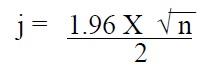
Or when n is odd
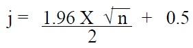
In both formulas, n is the sample size and j is an intermediate value that will be rounded to the next whole number.
By counting both up and down, using the rounded number from the median sales ratio, it can be stated with 95 percent confidence that the median sales ratio lies between these ratios. If the number of ratios in the sample is odd, count up and down beginning with ratios adjacent to the median ratio.
More specific information on the calculation and uses of the standard deviation, coefficient of variation, and confidence intervals can be found in the appraisal text titled Property Appraisal and Assessment Administration, 1990, IAAO. These same procedures can also be found in basic statistics texts at the local library.
State Board Performance Standards
In Colorado, all assessors are required to meet certain minimum statistical performance standards in appraising properties. The State Board of Equalization (state board) has adopted minimum statistical assessment standards and requires all assessors to achieve these standards for each assessment year. The standards are included in Addendum 8-A, State Board Compliance Requirements.
Failure to meet these standards may result in the following:
- A state board order for reappraisal.
- Reimbursement of state expenses relating to the cost of state supervision or assistance in implementing the state board ordered reappraisal.
- Pay back of any excess state aid to schools caused by an incorrect assessment level.
If additional information is needed about the understanding and use of statistics in mass appraisal, please refer to the Property Appraisal and Assessment Administration, 1990, and Standard On Ratio Studies, 2010, published by the International Association of Assessing Officers.
Addendum 8-A, State Board Compliance Requirements
The equitable and fair valuation of property requires the use of statistical analysis to monitor assessment level, uniformity, and assessment bias. The following requirements, recommendations, and optional measures are standards adopted by the State Board of Equalization (state board) and are benchmarks followed by the one percent assessment auditor. In addition, the information will assist the assessor in determining whether or not equitable and fair valuations have been achieved during a reappraisal.
Required Methodology
- All property classes and subclasses to be reappraised must be stratified by economic area. The state board's intent is written justification.
- The county must prepare a physical map(s) delineating economic areas resident in the county and the justification therefore. Each neighborhood associated with an economic area must be illustrated on a physical map.
- The county must, through computerization, appraisal records, or other means, be able to identify each property within the economic areas. Each property must be geographically identified by only one neighborhood and associated economic area. Economic areas are to be determined by analysis of homogeneous property characteristics, i.e., similar age, size, design, quality, sale price per square foot, etc.
- The number of observed sales ratios within each sample must meet or exceed the following sample requirements.
- An absolute minimum of 30 sales or appraisal ratios are required in each economic area or temporarily combined economic areas. The greatest number of calculated sales ratios available, given the constraints of sales data, time, and manpower, is recommended to be collected and analyzed.
- If 30 or more observed sales ratios are not available for a strata of property, the strata must be collapsed into a subclass. If insufficient ratios exist within a subclass, the subclass must be collapsed into a class. And if insufficient ratios exist within a class in a county, the sample for that class must be supplemented by sales and property characteristics from that class from a neighboring county.
State Board Statistical Compliance Requirements
- The assessment level of a reappraisal program must meet or exceed the following measures of level of value about the median sales ratio. The instructions for completing a median sales ratio calculation can be found earlier in this chapter.
- a. Vacant Land: 0.95 to 1.05
- Residential: 0.95 to 1.05 (Including condos and mobile homes)
- Commercial: 0.95 to 1.05
- Industrial: 0.95 to 1.05
- Agricultural: 0.90 to 1.10 (Including land, residences, but not support structures)
- Personal Prop.: 0.90 to 1.10 (Includes all personal property)
- Other: None
- The assessment quality of a reappraisal program must meet or exceed uniformity in values as measured by the coefficient of dispersion. The instructions for completing a coefficient of dispersion can be found earlier in this chapter.
- Vacant Land: 20.99 or less
- Residential: 15.99 or less (Including condominiums and mobile homes)
- Commercial: 20.99 or less
- Industrial: 20.99 or less
- Agricultural: 20.99 (Includes only Ag residences)
- Other: None
State Board Procedural Compliance Requirements
Subclasses to be subject to the assessment audit must include at least 20 percent of the valuation
of a class of property, unless otherwise noted.
- Vacant Land (All)
- Vacant land is eligible and may be subject to present worth valuation procedures established by the Division.
- Minimum number of parcels for a vacant land assessment audit in a county is 1,200.
- Residential (All)
- Only the market approach to appraisal is to be used.
- Commercial/Industrial (All)
- Cost, market, and income approaches to appraisal are to be used.
- Agricultural Land
- Use Chapter 5, Valuation of Agricultural Land, including current published base crops, expenses, and commodity prices.
- Use typical local expenses, which are documented and conform to the requirements found in Chapter 5, Valuation of Agricultural Land.
- Use NRCS soil surveys (if available) to identify classes of lands based on productivity capabilities.
- Use CASS yields and establish current crop rotation practices per CASS planted acreage.
- All expenses, income, yields, and cropping practices must reflect ten-year averages.
- Use statutory capitalization rate of 13 percent.
- Agricultural Residences
- Value is to be established using Chapter 5, Valuation of Agricultural Land, Agricultural Residential Improvements procedure for residences abstract coded as 4277, i.e., in the absence of sales data to the contrary, no adjustment factor other than factors applied to residences near city or town boundaries are to be used.
- Support (Rural) Structures
- Use Division procedures for valuing rural structures coded as 4279. Use standard inventory procedures and use only the cost approach to appraisal.
- Account for all structures whether salvage value has been applied or not.
- Natural Resources (All)
- Use Chapter 6, Valuation of Natural Resources, a random procedural check of a minimum of three schedules will be performed during the assessment audit.
- Personal Property (All)
- Use ARL VOLUME 5, PERSONAL PROPERTY MANUAL, including current discovery, classification, and documentation procedures, and including current economic lives table, cost factor tables, depreciation table, and level of value adjustment factor table.
- The county audit plan should be updated each year. The county audit plan must be feasible considering the county resources. The county will be evaluated by the independent auditor on the time schedule and adequacy of the audit plan.
- Aggregate ratio will be determined solely from the personal property accounts which have been physically inspected. The minimum assessment audit sample is 30 audited schedules (accounts). The level of value (median appraisal ratio) for personal property schedules analyzed must be between 90 and 110 percent.
State Board Supplemental Statistical Tests
The following statistical measures are not required by the state board, but are recommended as supplemental tests to provide additional confidence in appraised values.
- The assessment level of a reappraisal program should meet or exceed the following measures of level of value about the mean and aggregate (weighted) mean sales ratios. The instructions for completing a mean and weighted mean sales ratio can be found earlier in this chapter.
- Mean
- Vacant Land: 0.95 to 1.05
- Residential: 0.95 to 1.05
(Including condominiums and mobile homes) - Commercial: 0.95 to 1.05
- Industrial: 0.95 to 1.05
- Agricultural Except Support Structures 0.90 to 1.10
(Includes land, residences, and "other Ag." property)
- Aggregate (weighted) Mean
- Vacant Land: 0.95 to 1.05
- Residential: 0.95 to 1.05
(Including condominiums and mobile homes) - Commercial: 0.95 to 1.05
- Industrial: 0.95 to 1.05
- Agricultural Except Support Structures 0.90 to 1.10
(Includes land, residences, and "other Ag." property)
- Mean
- The assessment quality of a reappraisal program should achieve uniformity in values as demonstrated by meeting or exceeding the following measures of the Coefficient of Variation. Instructions for completing a coefficient of variation analysis can be found earlier in this chapter.
- Coefficient of Variation
- Vacant Land: 24.99 or less
- Residential: 19.99 or less
(Including condominiums and mobile homes) - Commercial: 24.99 or less
- Industrial: 24.99 or less
- Agricultural: 24.99 or less
(Includes residences)
- Coefficient of Variation
- The values within a class or subclass of property should exhibit a lack of bias against
lower or higher valued properties as measured by meeting or exceeding the following
measures of the Price-Related Differential as specified in Property Appraisal and
Assessment Administration, IAAO (1990) pg. 541. Instructions for completing a price
related differential can be found earlier in this chapter.- Residential: 0.98 to 1.03
- Commercial: 0.98 to 1.03
- Industrial: 0.98 to 1.03
Optional Statistical Tests
There are additional statistical tests that are available. More detailed instructions regarding the following optional tests can be found in the published text of Property Appraisal and Assessment Administration, 1990, IAAO.
- Other measures of assessment level include the following:
- Binomial Test - This test is to be used when sample size is less than 100. This test compares the number of observations actually falling in each of two categories with the number expected to fall in each category under the assumption that a stated hypothesis is true. The median appraisal ratio divides the number of observed sales ratios into two equal parts, to determine the correct level of value.
- Mann-Whitney Test - This test is an excellent non-parametric test of the null hypothesis that two classes or economic areas are assessed at the same percentage of market value, to measure the differences in level of assessment. This test seeks to determine whether the differences between two economic areas or classes are at the correct level of value.
- Kruskal-Wallis Test - This is a test that compares three or more property groups, e.g., economic areas or classes, to determine if they are assessed at equal percentages of market value, to measure differences in level of assessment. This test is similar to the Mann-Whitney Test.
- Other measures of bias or progressivity and regressivity include the following:
- Spearman Rank Test - This test statistically determines, at a specified confidence level, whether there is assessment bias. It uses both sales prices and assessment ratios that are ranked in order of magnitude from smallest to largest.
- Regression Analysis - This is probably the most effective means of detecting a systematic relationship between the level of assessment and property values. However this is a parametric test, which will yield a precise and effective measure of biases. Regression analysis and its corresponding results should be used with caution.
- Other measures of normality of assessment ratios include the following:
- Binomial Test for Normality - This test is to be used when sample size is less than 100. This test compares the number of observations actually falling in each of two categories. For example, ratios around the median should fall equally above and below the median if normally distributed.
- Chi Square Test for Normality - This test is to be used when sample size is greater than 100. This test detects non normal distributions when the data are skewed either to the left or to the right of the median.
- Other measures of reliability include the confidence interval. This test measures the degree of confidence that is specified in order to reject the null hypothesis. The null hypothesis, according to state board guidelines, is that the median assessment level is between 0.95 to 1.05. The test is to determine if this is true. A 95 percent confidence level means that one will accept the level as correct unless, after testing, it can be said with 95 percent confidence that it is not true.
Auditor's Supplemental Tests
Comparison of Sold and Unsold Parcels
The contractor will examine at least one percent of the assessment records in each county in order to compare the assessment levels of the properties listed in the market analysis with the valuations of other similar but unsold properties. The results of this analysis will be compiled in a manner that will identify whether the level of assessment for such properties has been adjusted in the same manner as for those properties for which sales data was available in the time period for obtaining the appropriate data.
Supplemental Appraisals
In no event can a sales ratio be established or utilized for any class or subclass of property unless there have been at least thirty sales, as required by § 39-1-103(8)(d), C.R.S. Whenever the sales sample for a specific class or subclass of property is less than 30 sales, the contractor will conduct independent appraisals of the identified class or subclass of property. The appropriate approaches to value, depending on the classification of the property, are utilized when completing the appraisals. In the event supplemental appraisals are necessary, appraisal ratios are calculated using the appraised values to ensure the results adequately reflect the accepted level of value and conforms to state board compliance requirements.
State Board Reappraisal Orders
Following are the guidelines considered by the state board when considering the issuance of reappraisal orders:
- A reappraisal will be ordered whenever the audit reveals the level of assessments falls outside the allowable range for the class or subclass of property in question. The median is the measure of central tendency used to measure the level of property value ratios.
- A reappraisal will be ordered whenever the audit results indicate the uniformity of assessments falls outside the allowable range for the class or subclass of property in question. The Coefficient of Dispersion is the measure of relative variability to determine the uniformity of value ratios.
- To measure the level and uniformity of sold and unsold properties, appraisals may be performed during the assessment audit to be used in appraisal ratio studies. These studies may determine if the assessor's appraised values are recommended for reappraisal orders, using the same standards as enumerated above for sales ratio studies.
- A reappraisal will be ordered, for the following year, if the abstract of assessment for any county which has completed an state board ordered reappraisal indicates values more than five percent below the values determined by the assessment audit. And, even if this five percent threshold has not been exceeded, the state board will order a reappraisal if the assessment audit shows the reappraisal was not consistent with the property tax provisions of the Colorado Constitution or statutes.
Assessor Requirements
- Provide neighborhoods/economic area boundary maps and computer codes to the assessment auditor.
- Provide current values and sales lists, by neighborhoods/economic area and for the entire county by class and subclass, for preliminary statistical compliance checks by the assessment auditor.
- Make value adjustments, as required for statistical compliance, prior to the final assessment audit report.
- Prepare the documentation to defend final values to the state board, if necessary.